The GlueX Beamline and Detector
Abstract:
The GlueX experiment at Jefferson Lab has been designed to study photoproduction reactions with a 9-GeV linearly polarized photon beam. The energy and arrival time of beam photons are tagged using a scintillator hodoscope and a scintillating fiber array. The photon flux is determined using a pair spectrometer, while the linear polarization of the photon beam is determined using a polarimeter based on triplet photoproduction. Charged-particle tracks from interactions in the central target are analyzed in a solenoidal field using a central straw-tube drift chamber and six packages of planar chambers with cathode strips and drift wires. Electromagnetic showers are reconstructed in a cylindrical scintillating fiber calorimeter inside the magnet and a lead-glass array downstream. Charged particle identification is achieved by measuring energy loss in the wire chambers and using the flight time of particles between the target and detectors outside the magnet. The signals from all detectors are recorded with flash ADCs and/or pipeline TDCs into memories allowing trigger decisions with a latency of 3.3 $\mu$s. The detector operates routinely at trigger rates of 40 kHz and data rates of 600 megabytes per second. We describe the photon beam, the GlueX detector components, electronics, data-acquisition and monitoring systems, and the performance of the experiment during the first three years of operation.Journal: NIM A 987 (2021) 164807
arXiv: arXiv:2005.14272
NIM A 987 (2021) 164807: downloads png pdf |
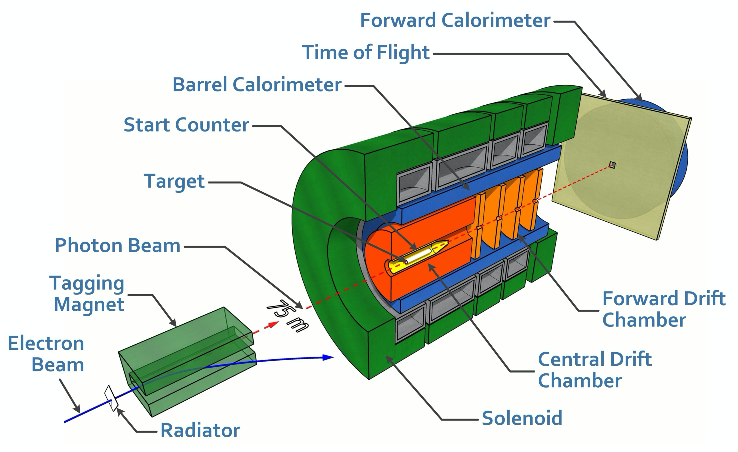
Figure 1:
A cut-away drawing of the GlueX detector in Hall D, not to scale. |
NIM A 987 (2021) 164807: downloads png pdf |
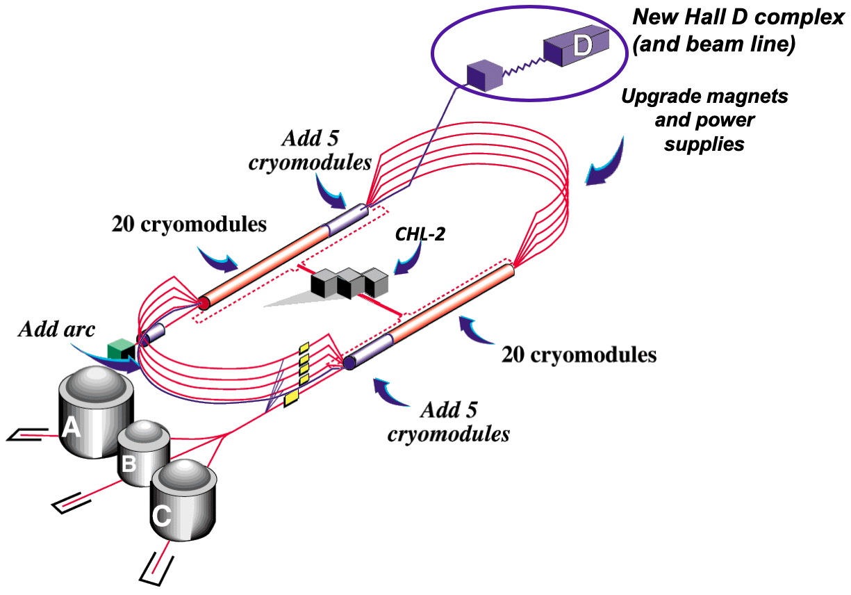
Figure 2:
Schematic of the CEBAF accelerator showing the additions made during the 12-GeV project. The Hall-D complex is located at the north-east end. |
NIM A 987 (2021) 164807: downloads png pdf |
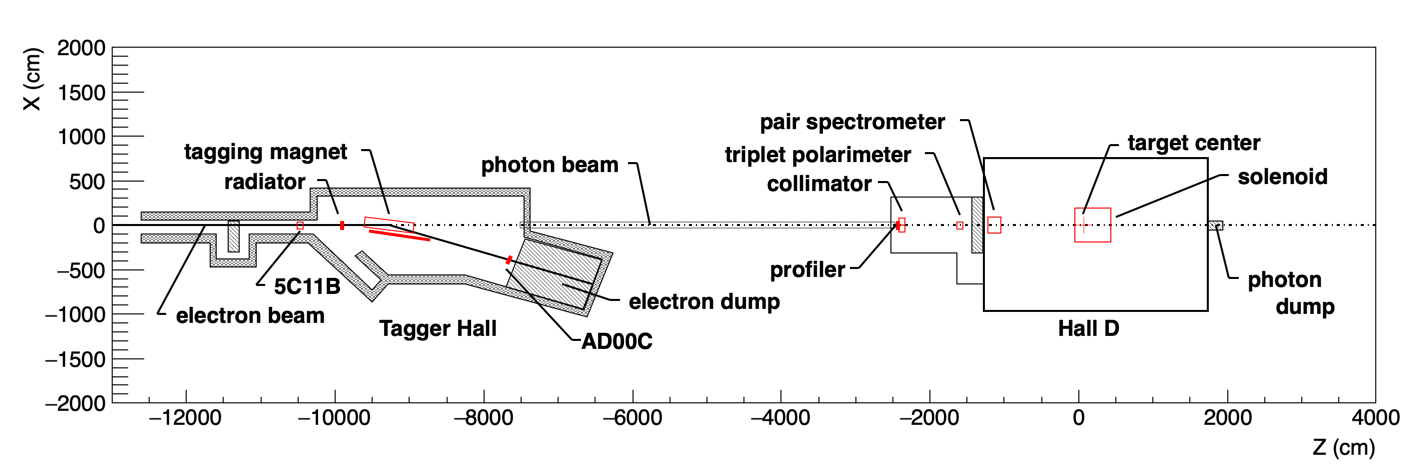
Figure 4:
Schematic layout of the Hall-D complex, showing the Tagger Hall, Hall D, and several of the key beamline devices. Also indicated are the locations of the 5C11B and AD00C beam monitors. |
NIM A 987 (2021) 164807: downloads png pdf |
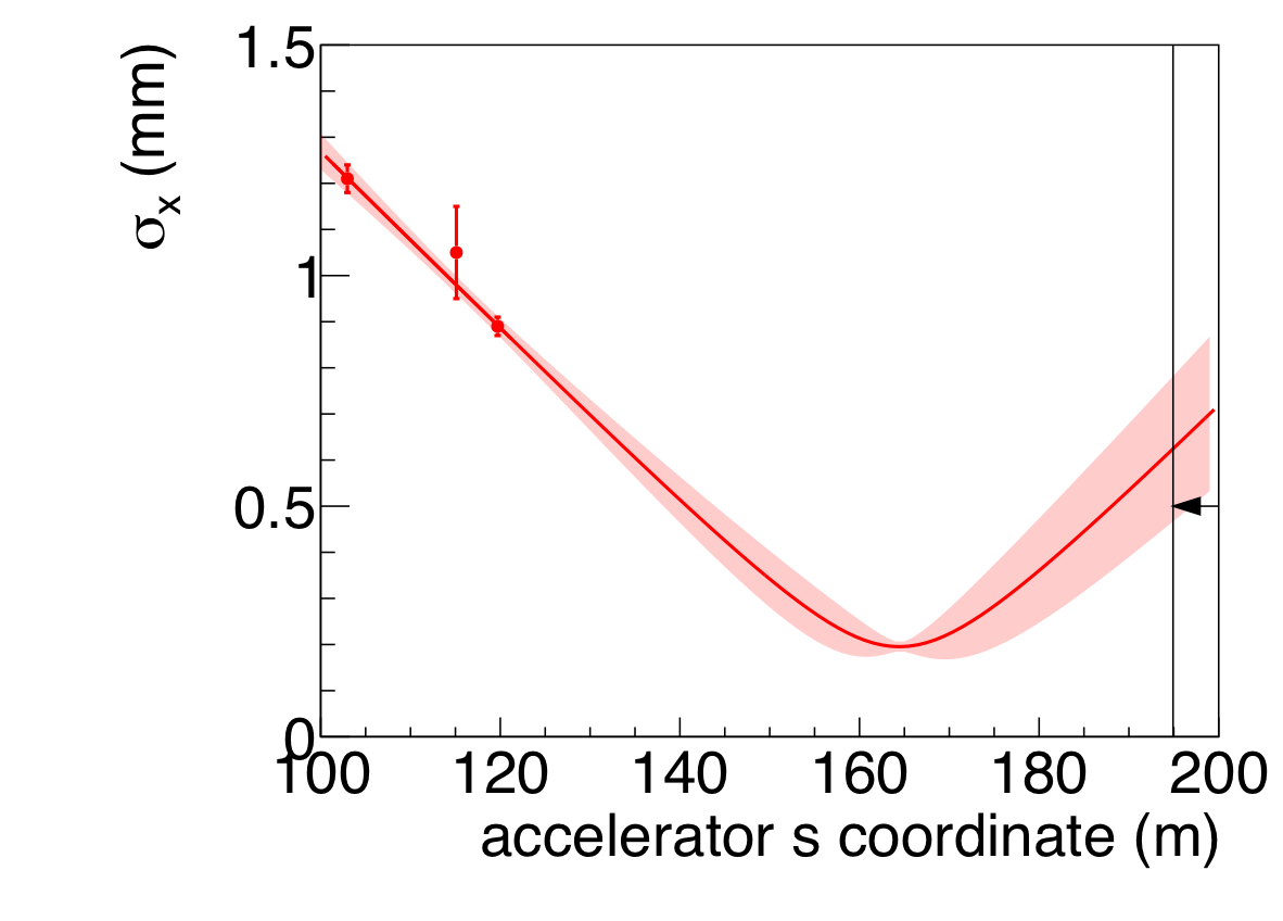
Figure 5a:
Measurements of the root-mean-square width of the electron beam in horizontal (left) and vertical (right) projections as a function of position along the beamline, based on harp scans (data points) of the electron beam. The radiator position is just upstream of the third data point. The primary collimator position is marked by the vertical line indicated by the arrow. The curve downstream of the radiator is an extrapolation from the measured data points, with extrapolation uncertainty indicated by the shaded regions. |
NIM A 987 (2021) 164807: downloads png pdf |
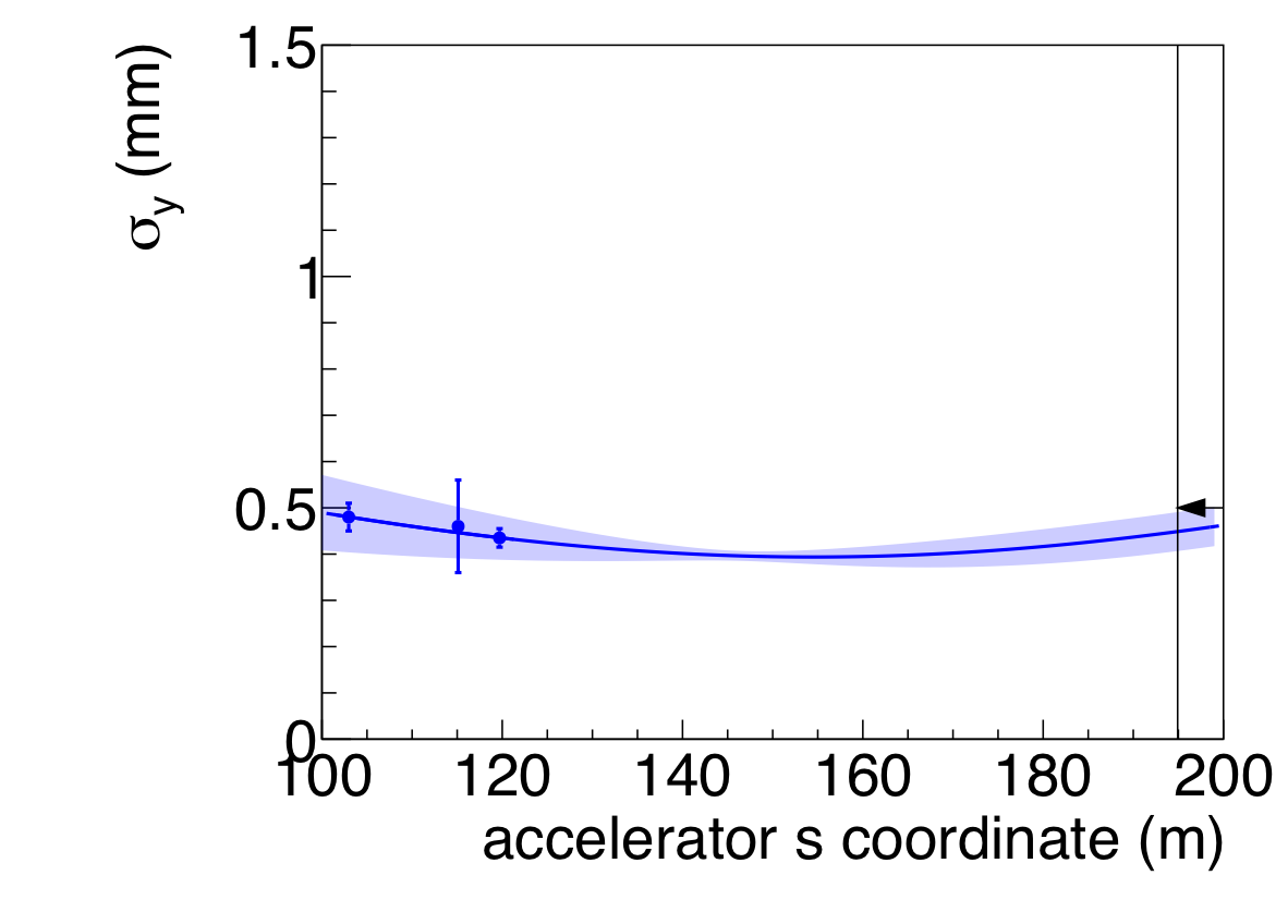
Figure 5b:
Measurements of the root-mean-square width of the electron beam in horizontal (left) and vertical (right) projections as a function of position along the beamline, based on harp scans (data points) of the electron beam. The radiator position is just upstream of the third data point. The primary collimator position is marked by the vertical line indicated by the arrow. The curve downstream of the radiator is an extrapolation from the measured data points, with extrapolation uncertainty indicated by the shaded regions. |
NIM A 987 (2021) 164807: downloads png pdf |
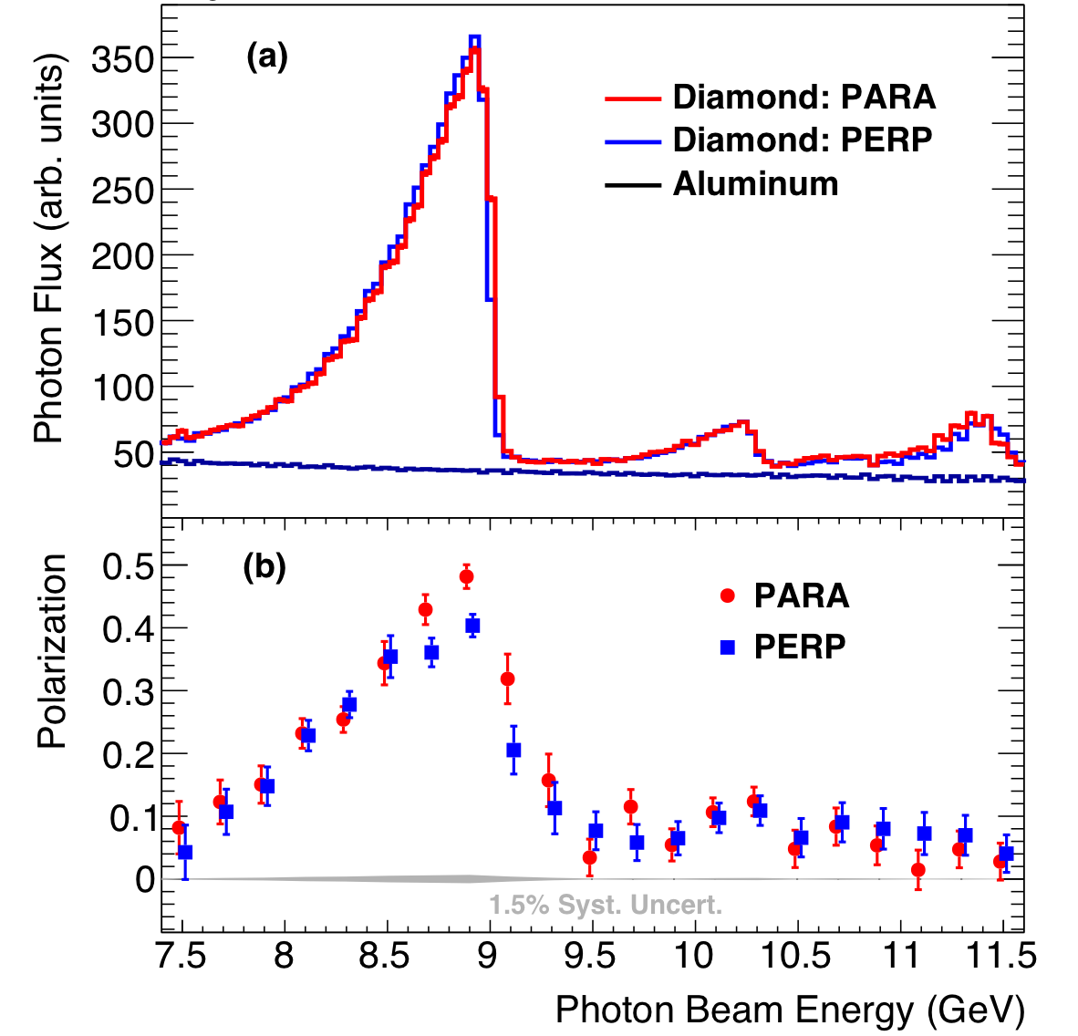
Figure 6:
(a) Collimated photon beam intensity versus energy as measured by the Pair Spectrometer. (b) Collimated photon beam polarization as a function of beam energy, as measured by the Triplet Polarimeter, with data points offset horizontally by $\pm0.015$ GeV for clarity. Thes that are parallel and perpendicular to the horizontal, respectively. |
NIM A 987 (2021) 164807: downloads png pdf |
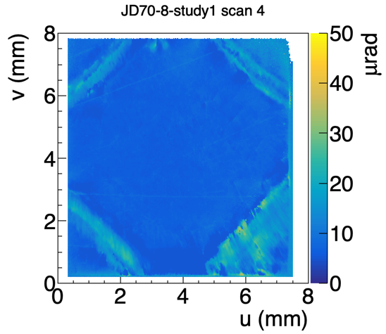
Figure 7:
Rocking curve RMS width topograph taken of the (2,2,0) reflection from a CVD diamond crystal using 15 keV X-rays at the C-line at CHESS. The bright diagonal lines in the corners indicate regions of increased local strain, coinciding with growth boundaries radiating outward from the seed crystal used in the CVD growth process. |
NIM A 987 (2021) 164807: downloads png pdf |
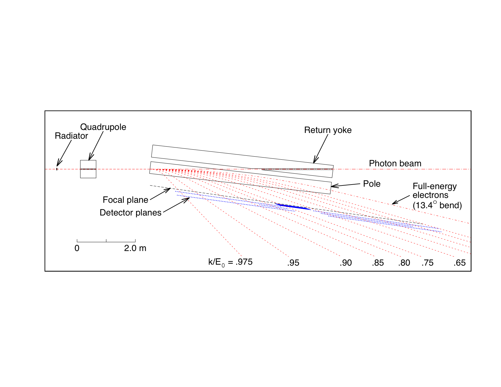
Figure 8:
Schematic diagram of the tagging spectrometer, showing the paths of the electron and photon beams. Dotted lines indicate post-radiation electron trajectories identified by the energy the electron gave up to an associated radiated photon, as a fraction of the beam energy E$_0$. The Tagger focal plane detector arrays TAGH and TAGM are described in the text. |
NIM A 987 (2021) 164807: downloads png pdf |
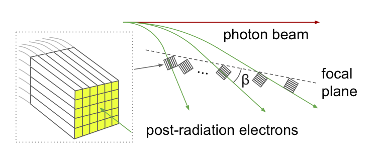
Figure 9:
Conceptual overview of the tagger microscope design, showing the fiber bundles and light guides (left), and the orientation of these bundles aligned with the incoming electron beam direction in the tagger focal plane (right). The variation of the crossing angle $\beta$ is exaggerated for the sake of illustration. |
NIM A 987 (2021) 164807: downloads png pdf |
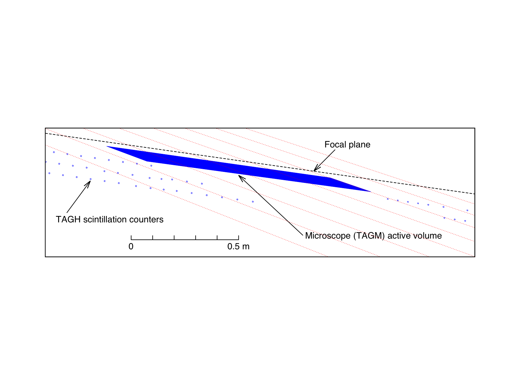
Figure 10:
Schematic of electron trajectories in the region of the microscope. Shown are the three layers of hodoscope counters on either side of the microscope and the region covered by the microscope. |
NIM A 987 (2021) 164807: downloads png pdf |
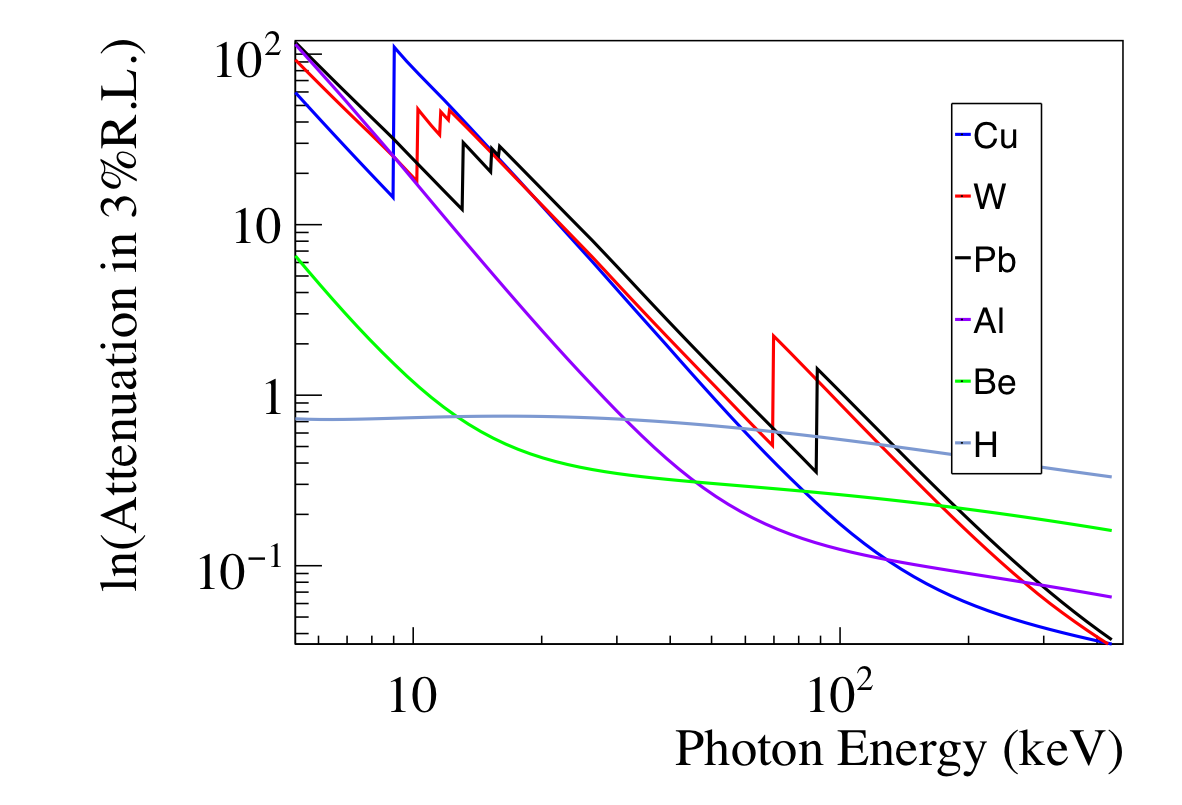
Figure 11:
Attenuation of low-energy photons in foils with a thickness of $3%$ of a radiation length for different materials as a function of photon energy. The W foil was selected to reduce the random background hits in the detector drift chambers. The attenuation coefficients are taken from Ref. [20] |
NIM A 987 (2021) 164807: downloads png pdf |
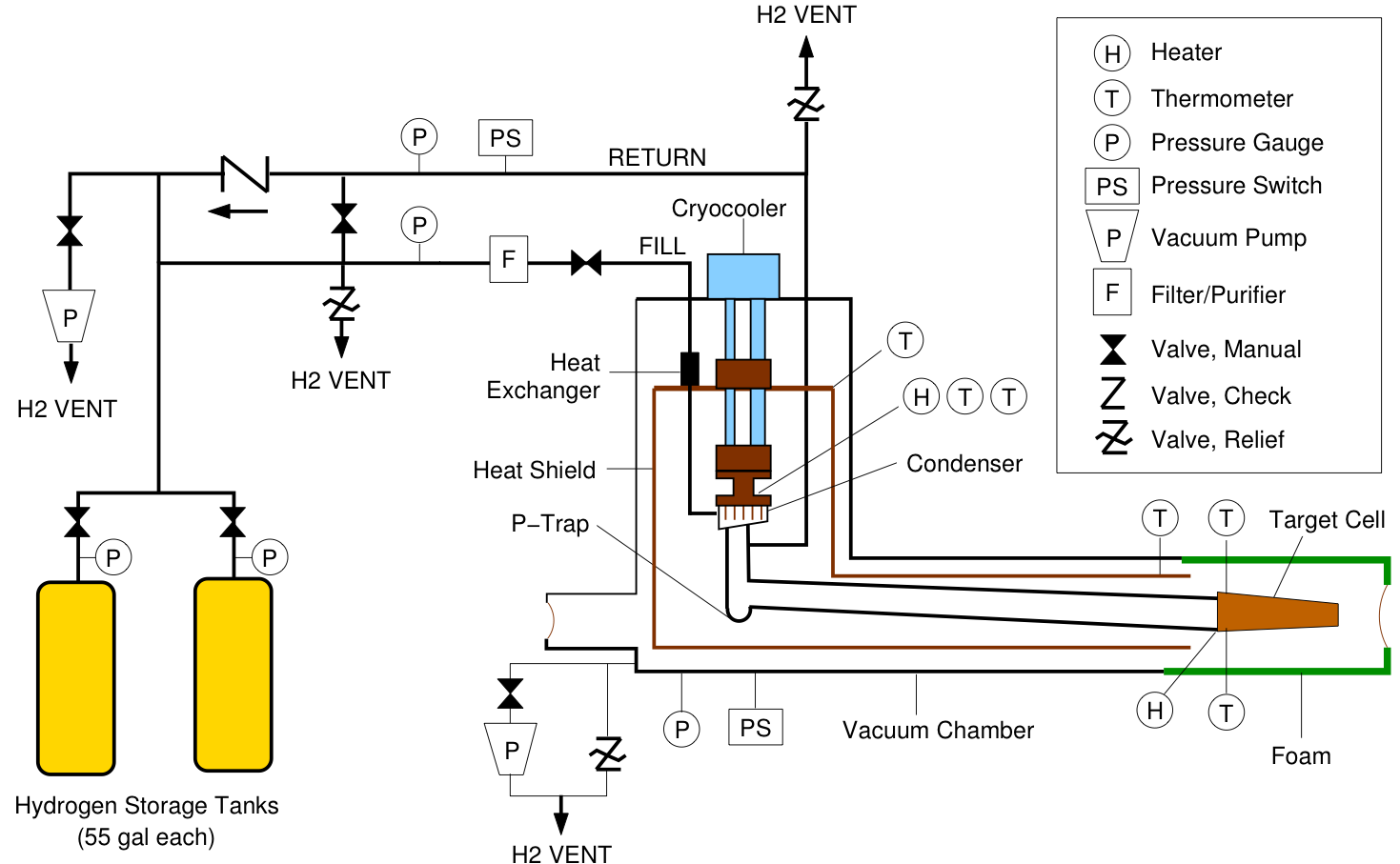
Figure 13:
Simplified process and instrumentation diagram for the GlueX liquid hydrogen target (not to scale). In the real system, the P-trap is above the level of the target cell and is used to promote convective cooling of the target cell from room temperature. |
NIM A 987 (2021) 164807: downloads png pdf |
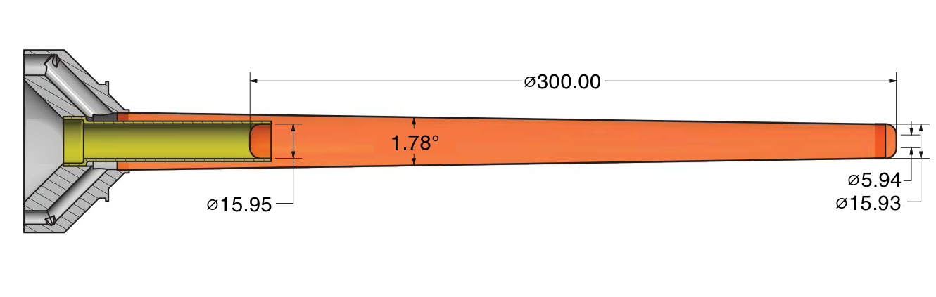
Figure 14:
Target cell for the liquid hydrogen target. Dimensions are in mm. |
NIM A 987 (2021) 164807: downloads png pdf |
Figure 15:
Cross-section through the cylindrically symmetric Central Drift Chamber, along the beamline. |

NIM A 987 (2021) 164807: downloads png pdf |
Figure 16:
The Central Drift Chamber during construction. A partially completed layer of stereo straw tubes is shown, surrounding a layer of straw tubes at the opposite stereo angle. Part of the carbon fiber endplate, two temporary tension rods and some of the 12 permanent support rods linking the two endplates can also be seen. |
NIM A 987 (2021) 164807: downloads png pdf |
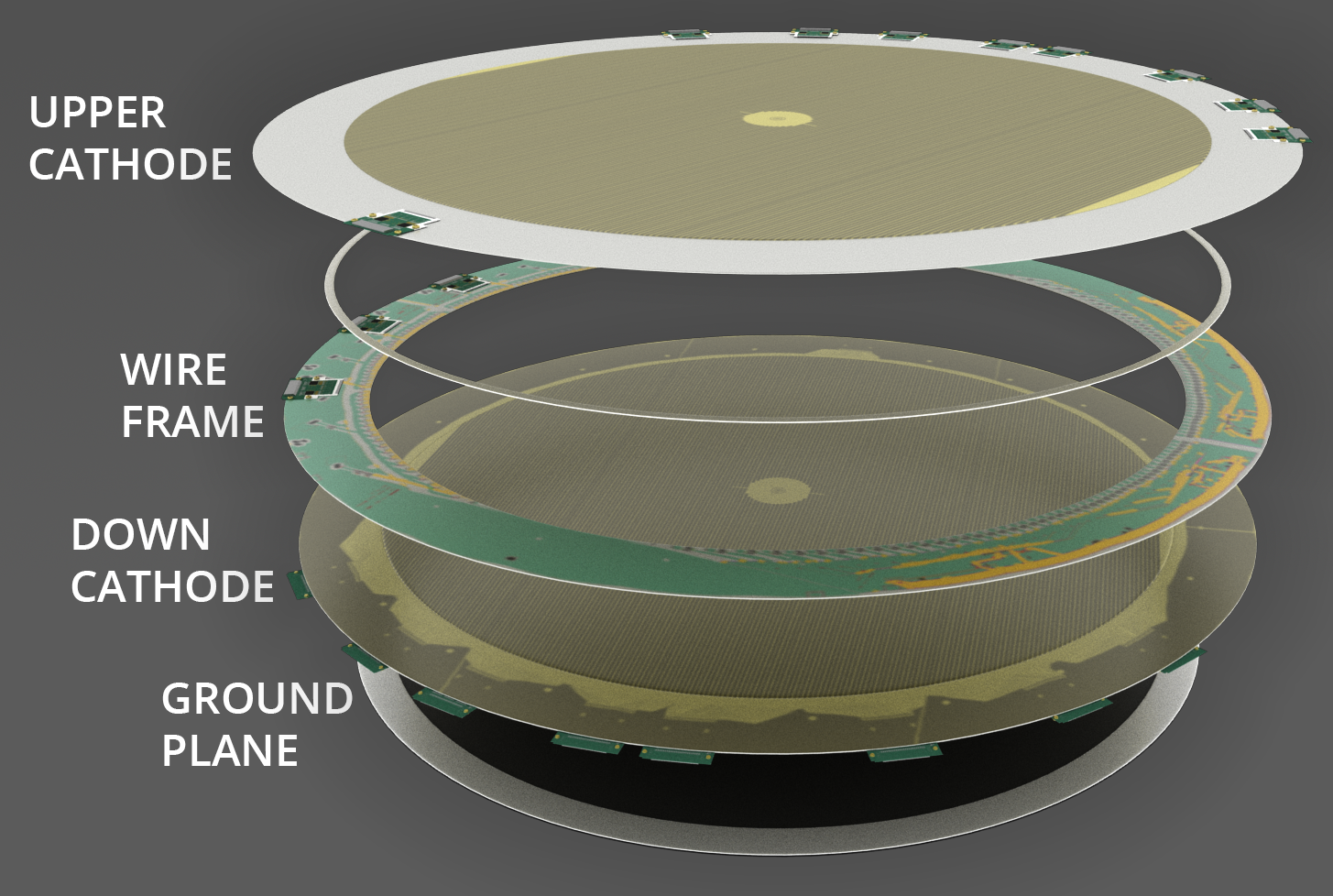
Figure 17:
Artist rendering of one FDC chamber showing components. From top to bottom, upstream cathode, wire frame, downstream cathode, ground plane that separates the chambers. The diameter of the active area is $1$ m. |
NIM A 987 (2021) 164807: downloads png pdf |
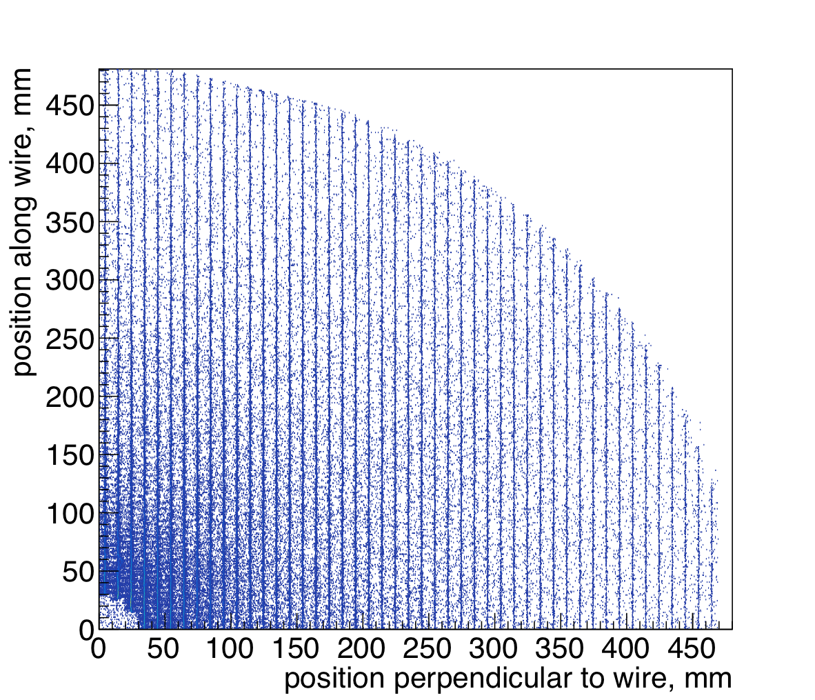
Figure 18:
Wire (avalanche) positions reconstructed from the strip information on the two cathodes in one FDC chamber. Only one quarter of the chamber is shown in this figure. |
NIM A 987 (2021) 164807: downloads png pdf |
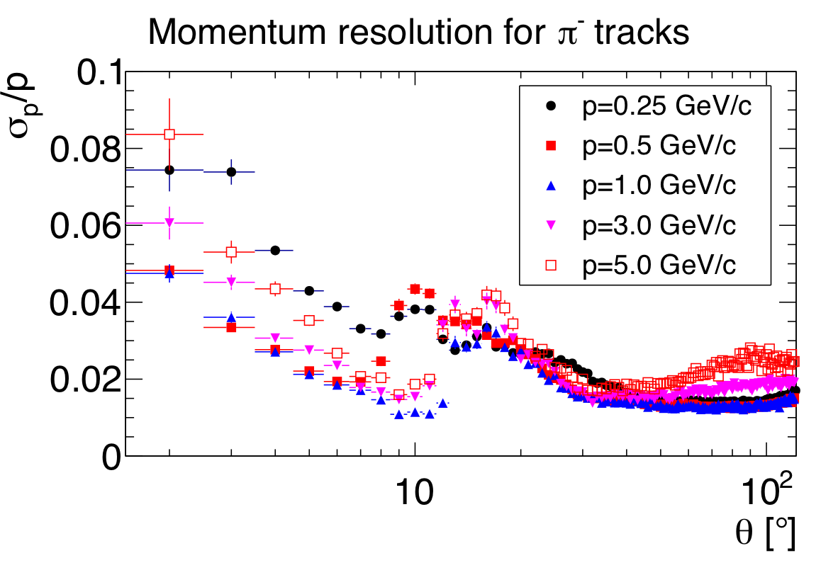
Figure 19a:
(Left) Momentum resolution for $\pi^-$ tracks. (Right) Momentum resolution for proton tracks. |
NIM A 987 (2021) 164807: downloads png pdf |
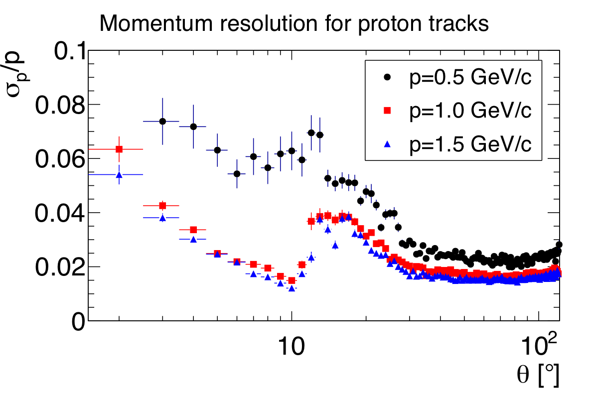
Figure 19b:
(Left) Momentum resolution for $\pi^-$ tracks. (Right) Momentum resolution for proton tracks. |
NIM A 987 (2021) 164807: downloads png pdf |
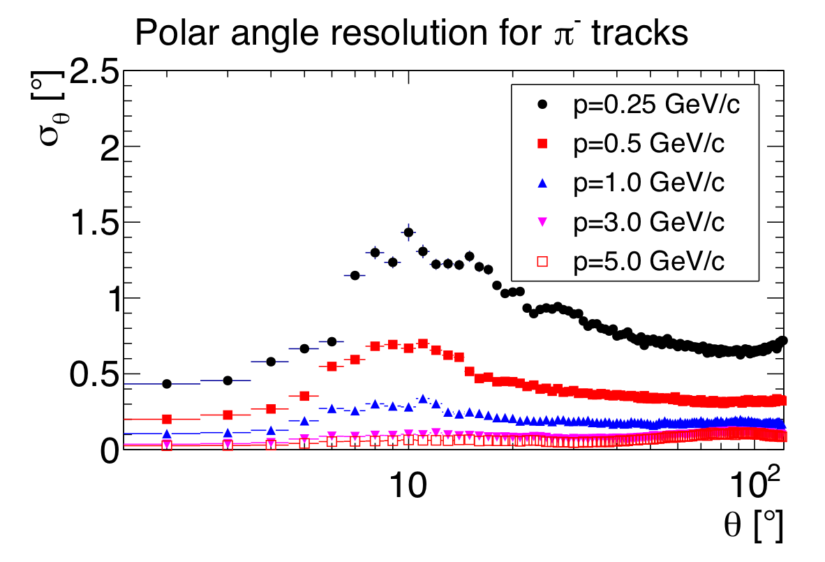
Figure 20a:
(Left) Polar angle resolution for $\pi^-$ tracks. (Right) Azimuthal angle resolution for $\pi^-$ tracks. The resolutions are plotted as a function of the polar angle, $\theta$. |
NIM A 987 (2021) 164807: downloads png pdf |
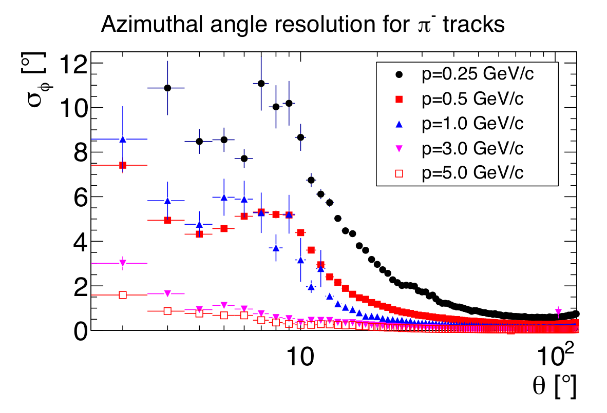
Figure 20b:
(Left) Polar angle resolution for $\pi^-$ tracks. (Right) Azimuthal angle resolution for $\pi^-$ tracks. The resolutions are plotted as a function of the polar angle, $\theta$. |
NIM A 987 (2021) 164807: downloads png pdf |
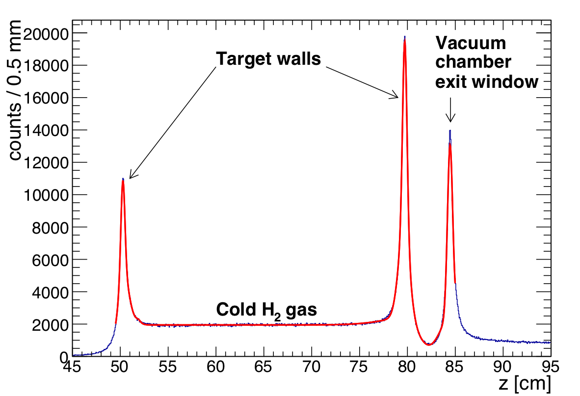
Figure 21:
Reconstructed vertex positions within 1 cm radial distance with respect to the beam line for an empty target measurement. The curve shows the result of a fit to the vertex distribution used to determine the vertex resolution. |
NIM A 987 (2021) 164807: downloads png pdf |
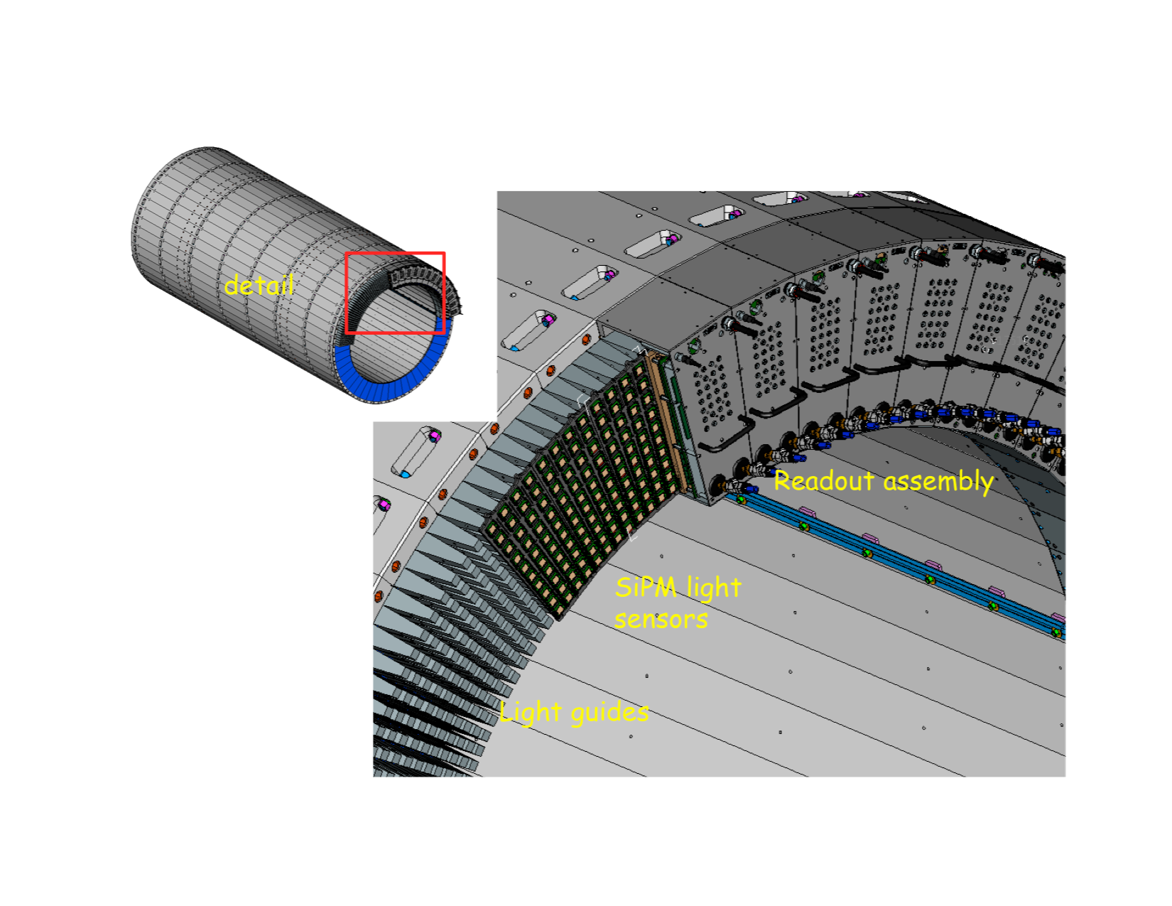
Figure 22:
Three-dimensional rendition of the light guides mounted at the end of the BCAL, as well as the readout assemblies mounted over them. The readout assemblies contain the SiPMs and their electronics. |
NIM A 987 (2021) 164807: downloads png pdf |
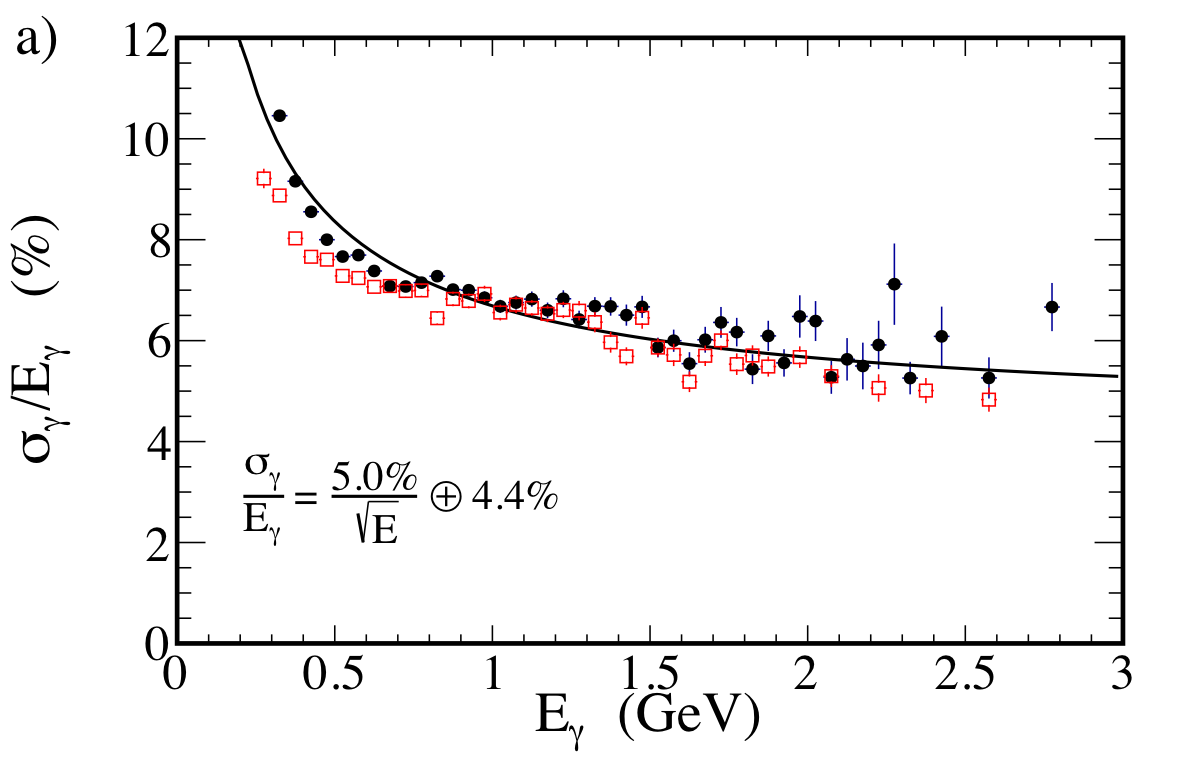
Figure 24a:
The energy resolution, $\sigma_\gamma/E_\gamma$, for single photons in the a) BCAL and b) FCAL calculated from the $\eta$ mass distribution under the assumption that only the energy resolution contributes to its width. Solid black circles are data and open red squares are simulation. Fitted curves including the stochastic and constant terms are indicated. |
NIM A 987 (2021) 164807: downloads png pdf |
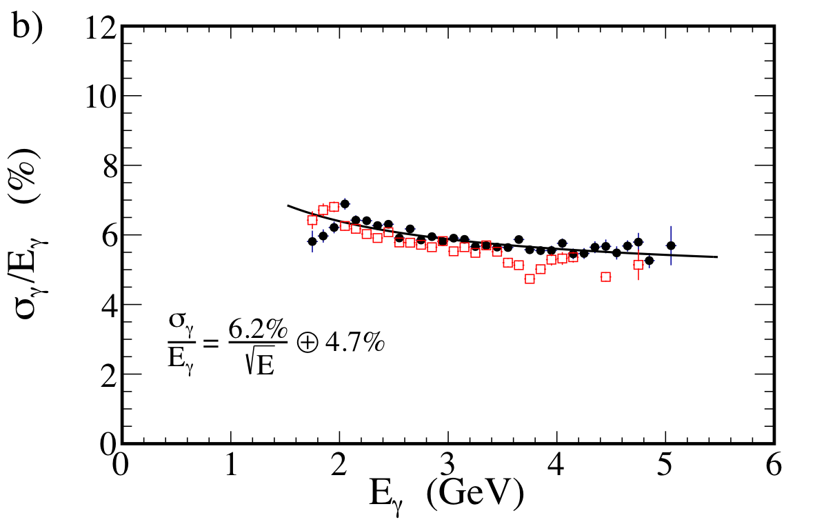
Figure 24b:
The energy resolution, $\sigma_\gamma/E_\gamma$, for single photons in the a) BCAL and b) FCAL calculated from the $\eta$ mass distribution under the assumption that only the energy resolution contributes to its width. Solid black circles are data and open red squares are simulation. Fitted curves including the stochastic and constant terms are indicated. |
NIM A 987 (2021) 164807: downloads png pdf |
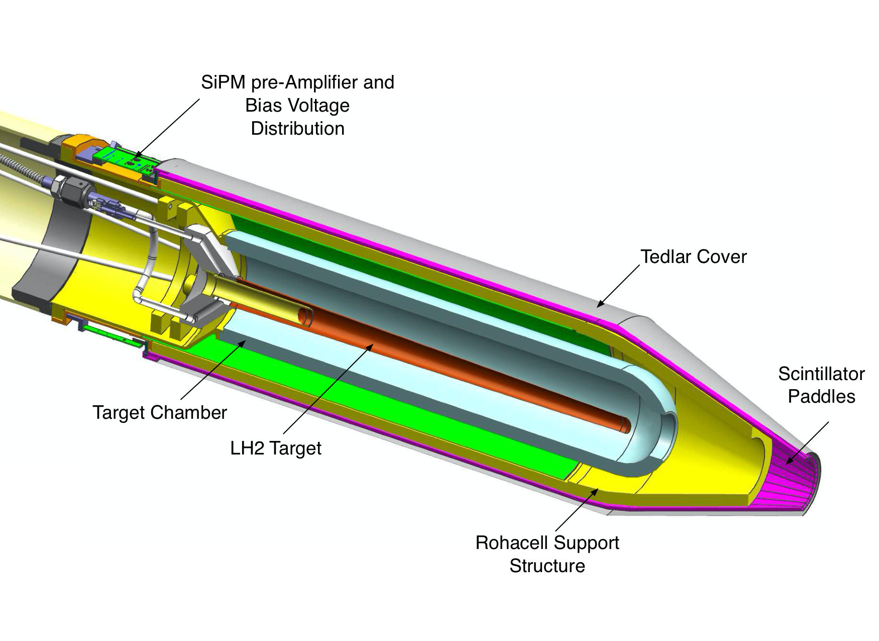
Figure 25:
The GlueX Start Counter surrounding the liquid-hydrogen |
NIM A 987 (2021) 164807: downloads png pdf |
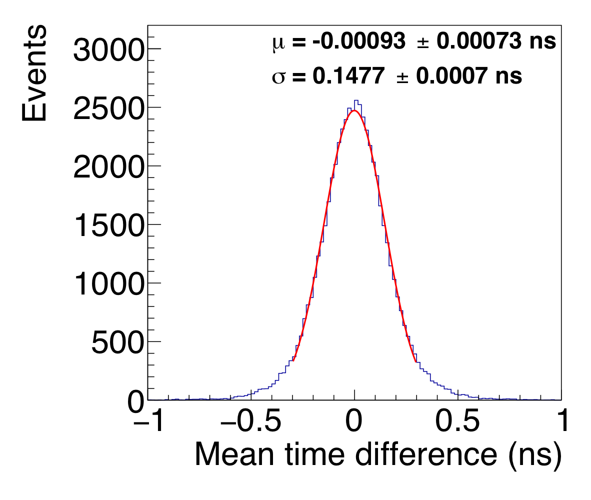
Figure 26:
Mean time difference between one TOF long paddle of one plane with all other long paddles of the other plane. |

NIM A 987 (2021) 164807: downloads png pdf |
Figure 27:
Time difference distribution between the vertex time computed from the start counter and the accelerator RF. The time from the RF does not contribute significantly to the width of the distribution. The fit function is a double Gaussian plus a third-degree polynomial. %The vertical lines indicate the cuts used to identify a 250 MHz beam bunch. |
NIM A 987 (2021) 164807: downloads png pdf |
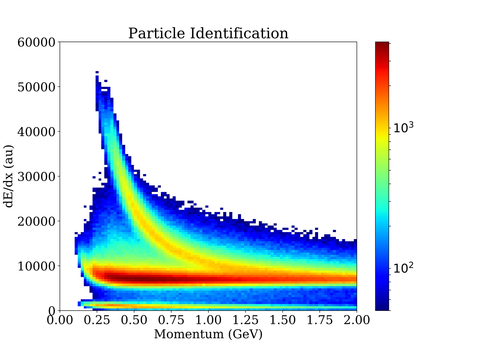
Figure 28:
$dE/dx$ vs.\ $p$ for the Start Counter. The curved band corresponds to protons while the horizontal band corresponds to electrons, pions, and kaons. Pion/proton separation is achievable |
NIM A 987 (2021) 164807: downloads png pdf |
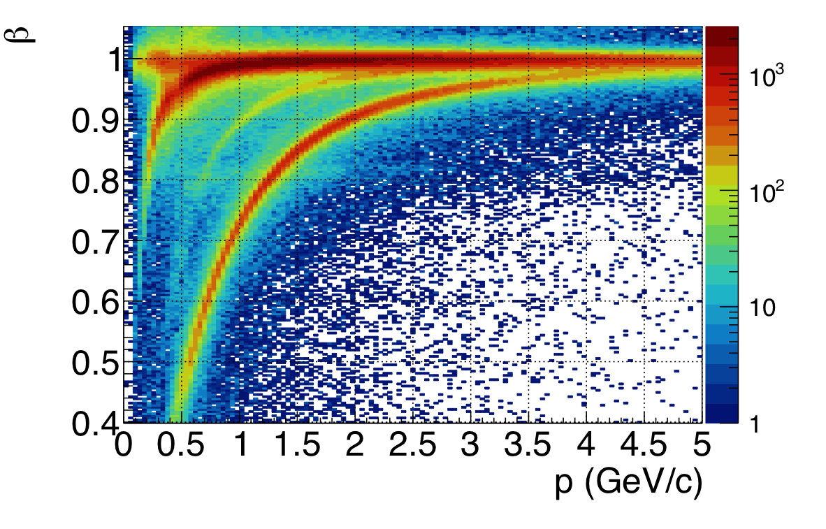
Figure 29:
$\beta$ of positive tracks versus track momentum, showing bands for $e^+$, $\pi^+$, $K^+$ and $p$ for the TOF detector. The color coding of the third dimension is in logarithmic scale. |
NIM A 987 (2021) 164807: downloads png pdf |
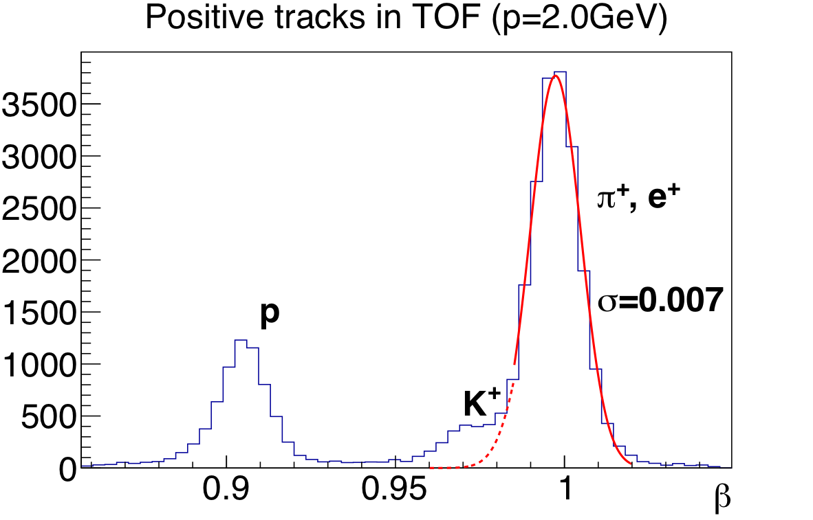
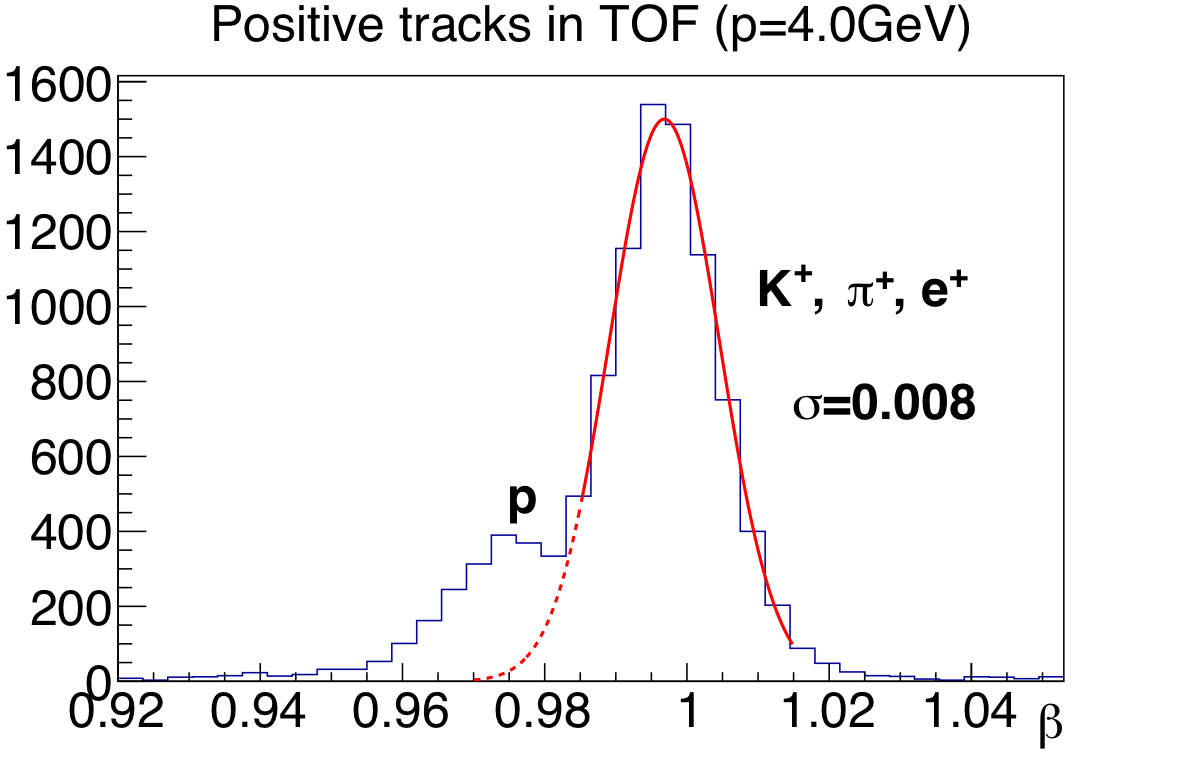
Figure 30a:
$\beta$ of positive tracks with 2 GeV/c momentum (left) and with 4 GeV/c (right). |
NIM A 987 (2021) 164807: downloads png pdf |
Figure 30b:
$\beta$ of positive tracks with 2 GeV/c momentum (left) and with 4 GeV/c (right). |
NIM A 987 (2021) 164807: downloads png pdf |
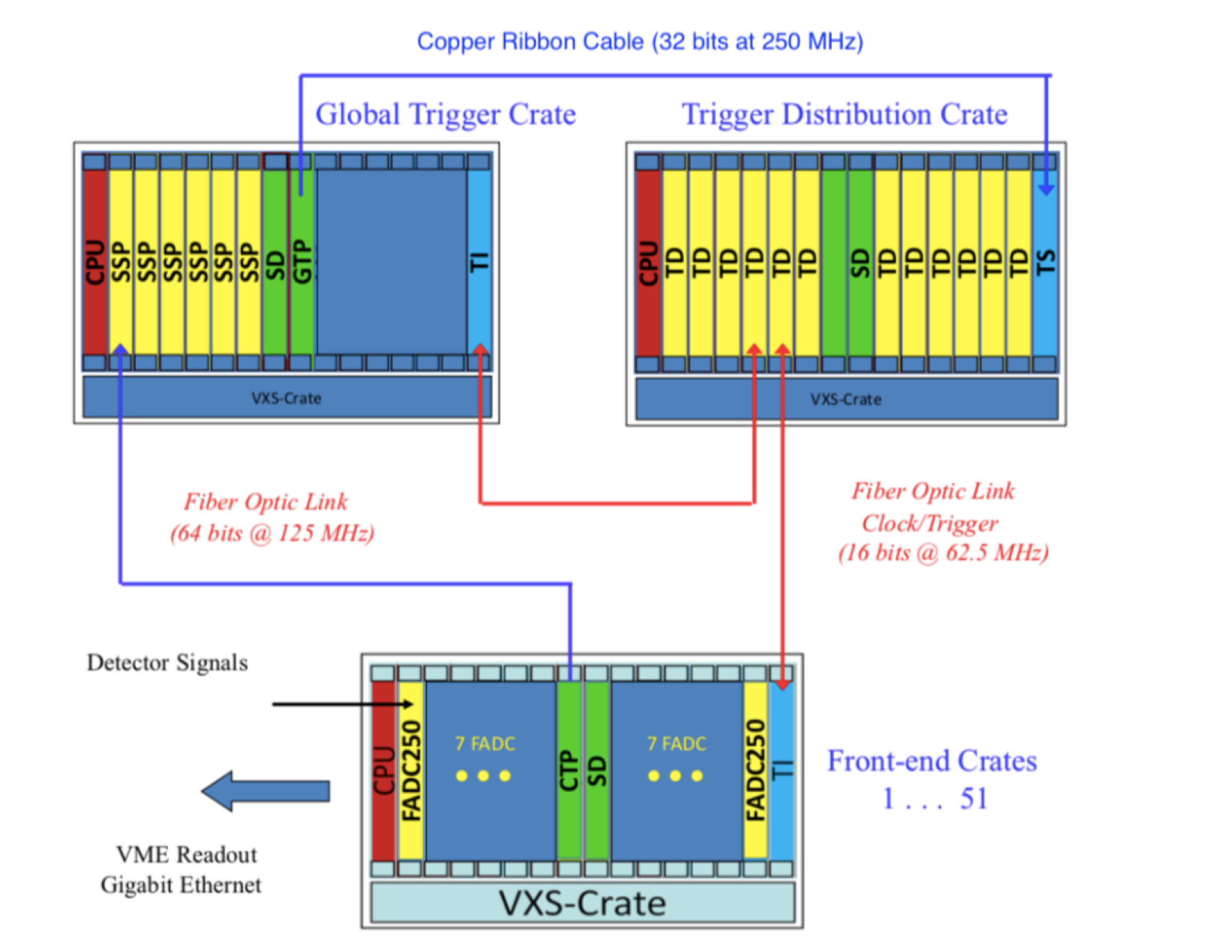
Figure 31:
Schematic view of the Level-1 trigger system of the GlueX experiment. The electronics boards are described in the text. |
NIM A 987 (2021) 164807: downloads png pdf |
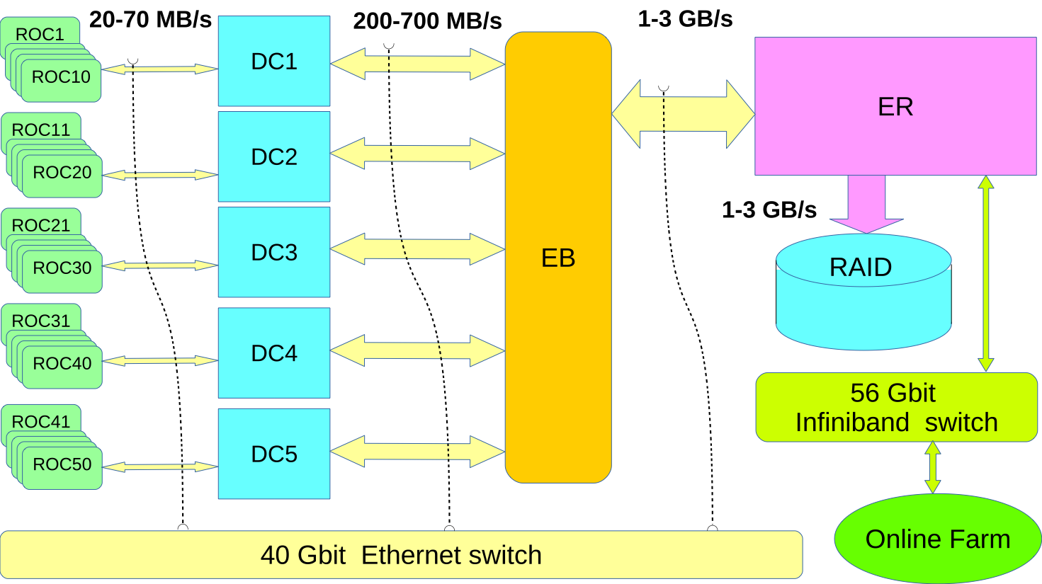
Figure 33:
Schematic DAQ configuration for GlueX. The high-speed DAQ connections between the ROCs and the ER are contained within an isolated network. The logical data paths are indicated by arrows, although physically they are routed through the 40 Gbit ethernet switch. The online monitoring system uses its own separate 56 Infiniband switch. |
NIM A 987 (2021) 164807: downloads png pdf |
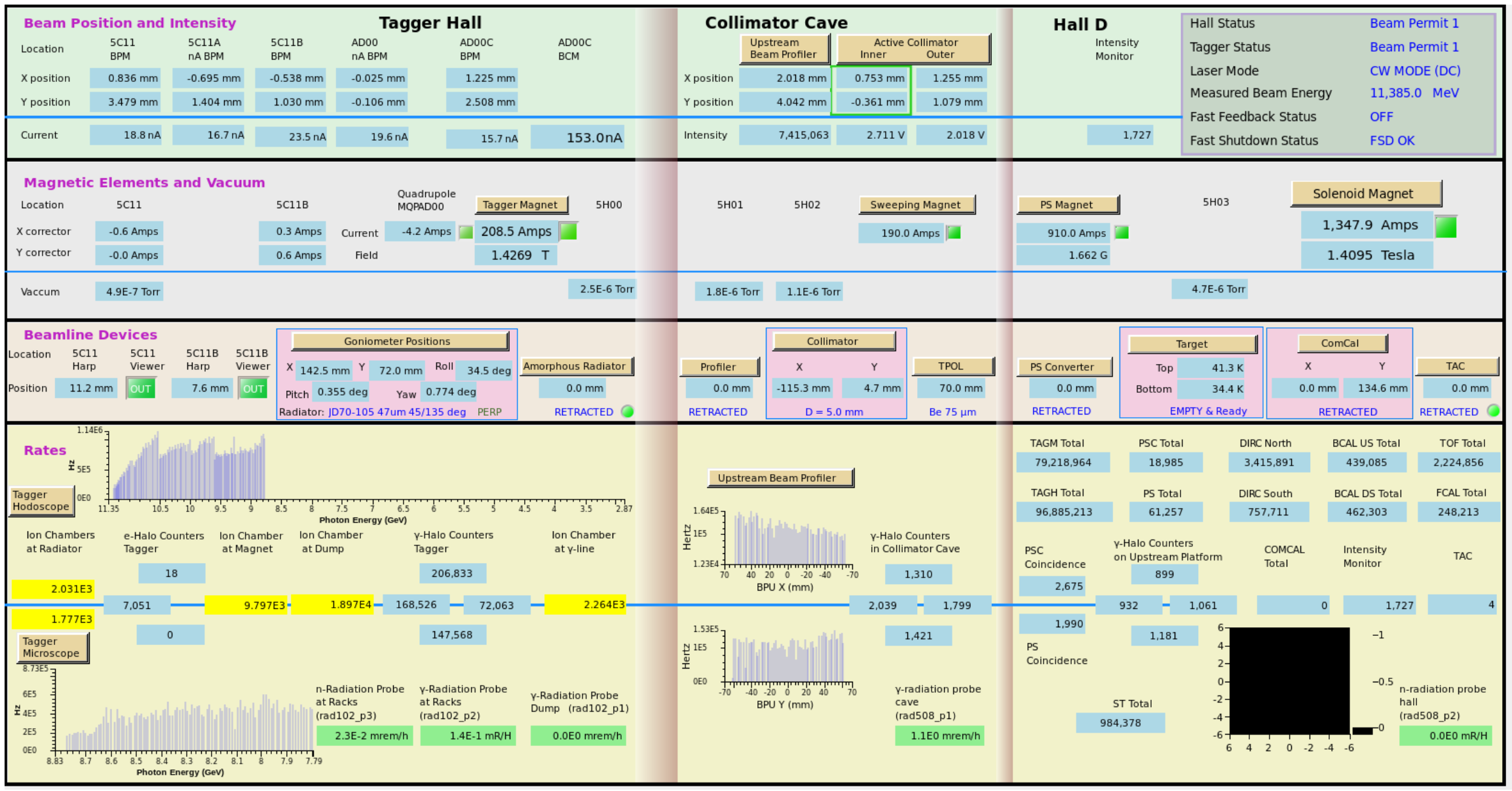
Figure 34:
Top-level graphical interface for the beamline. This screen provides information on beam currents and rates, radiators, magnet status, target condition, background levels, etc. |
NIM A 987 (2021) 164807: downloads png pdf |
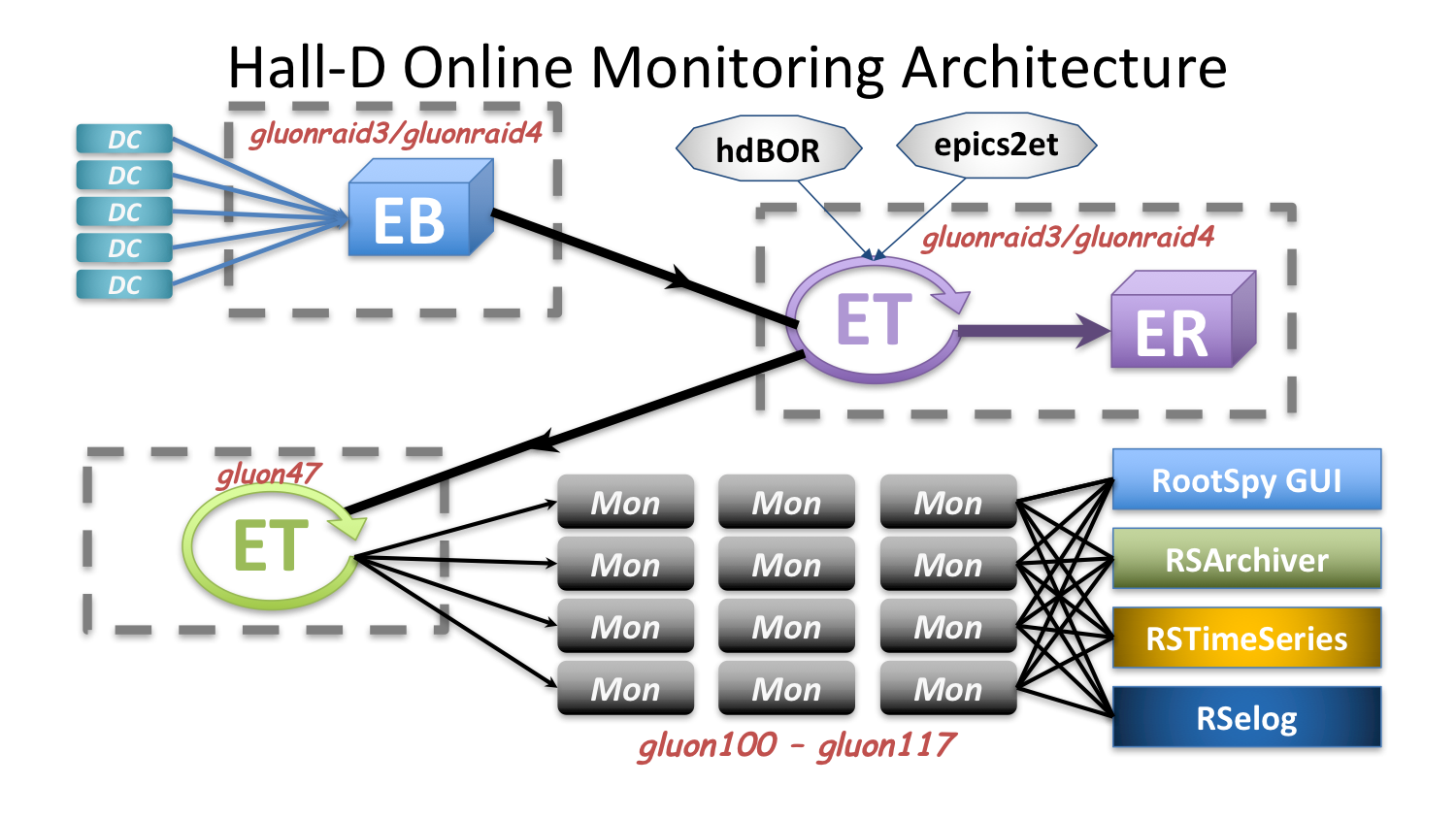
Figure 35:
Processes distributed across several computers in the online monitoring system. DC, EB, and ER are the Data Concentrator, Event Builder, and Event Recorder processes, respectively, in the CODA DAQ system. |

NIM A 987 (2021) 164807: downloads png pdf |
Figure 36:
Invariant mass distributions showing $\pi^\circ$, $\omega$, $\rho$, and $\phi$ particles. These plots were generated online in about 1hr 40min by looking at roughly 2% of the data stream. |

NIM A 987 (2021) 164807: downloads png pdf |
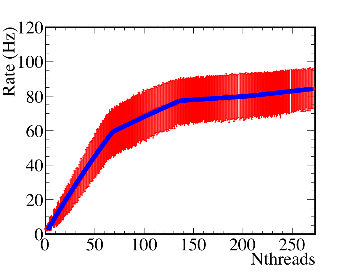
Figure 37:
The scaling of program performance as a function of the number of processing threads. The computer used for this test consisted of 24 full cores (Intel x86\_64) plus 24 hyperthreads. The orange squares are from running multiple processes, each with 12 threads. |
NIM A 987 (2021) 164807: downloads png pdf |
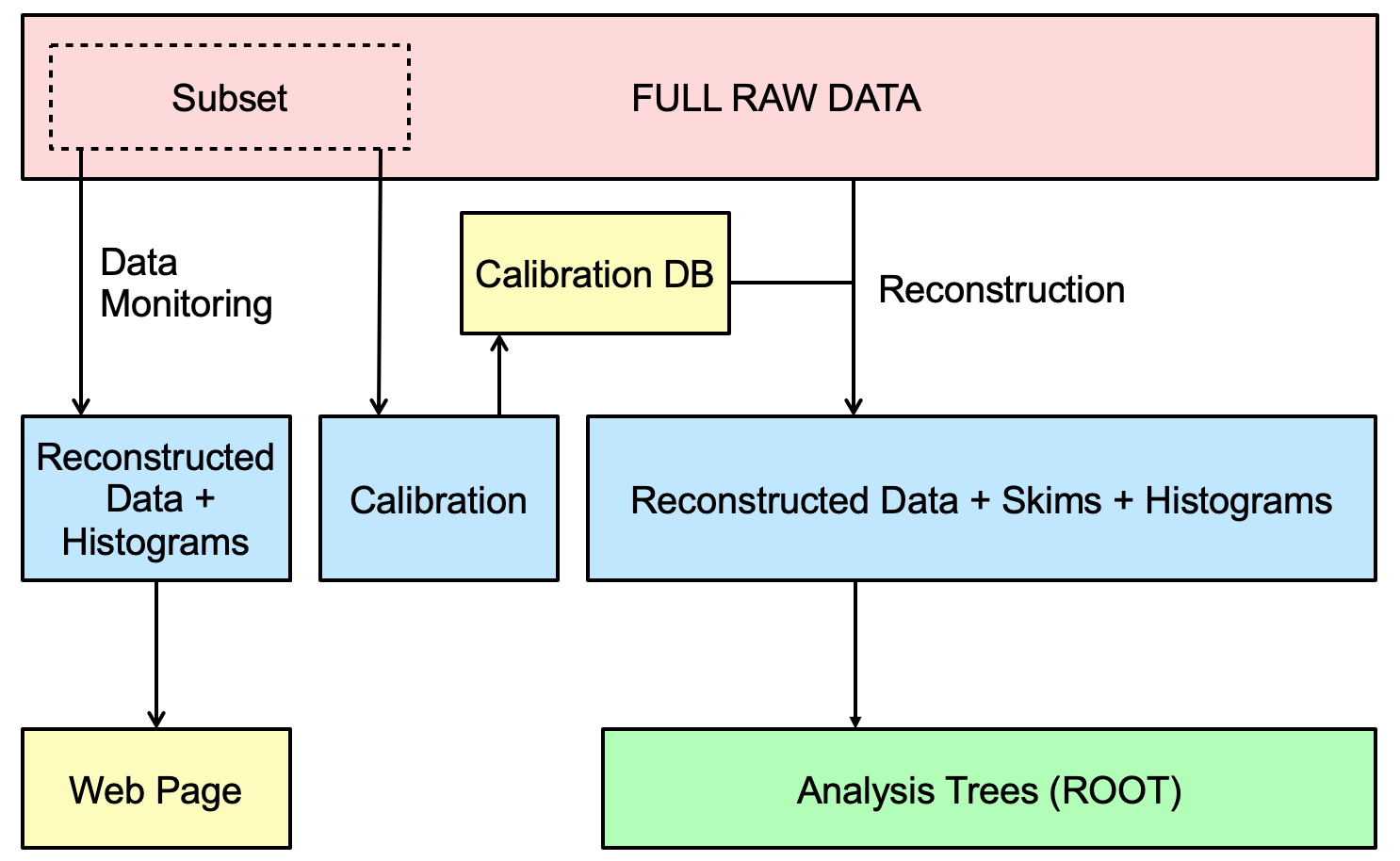
Figure 38:
Production flowchart for \GX data, illustrating analysis steps. |
NIM A 987 (2021) 164807: downloads png pdf |
Figure 39a:
Event processing rate versus number of threads for reconstruction jobs on NERSC Cori II (left) and PSC Bridges (right). The slope changes in the NERSC plot are due to the KNL architecture, which had four hardware threads per core. For PSC Bridges, hyper-threading is disabled and the plot shows a single slope. |

NIM A 987 (2021) 164807: downloads png pdf |
Figure 39b:
Event processing rate versus number of threads for reconstruction jobs on NERSC Cori II (left) and PSC Bridges (right). The slope changes in the NERSC plot are due to the KNL architecture, which had four hardware threads per core. For PSC Bridges, hyper-threading is disabled and the plot shows a single slope. |

NIM A 987 (2021) 164807: downloads png pdf |
Figure 40:
The Monte Carlo data flow from event generators through physics analysis REST files. The ovals represent databases containing tables indexed by run number, providing a common configuration for simulation, smearing, and reconstruction. Background events represented by the circle marked \emph{bg} are real events collected using a random trigger, which are overlaid on the simulated events to account for pile-up in the Monte Carlo. |
NIM A 987 (2021) 164807: downloads png pdf |
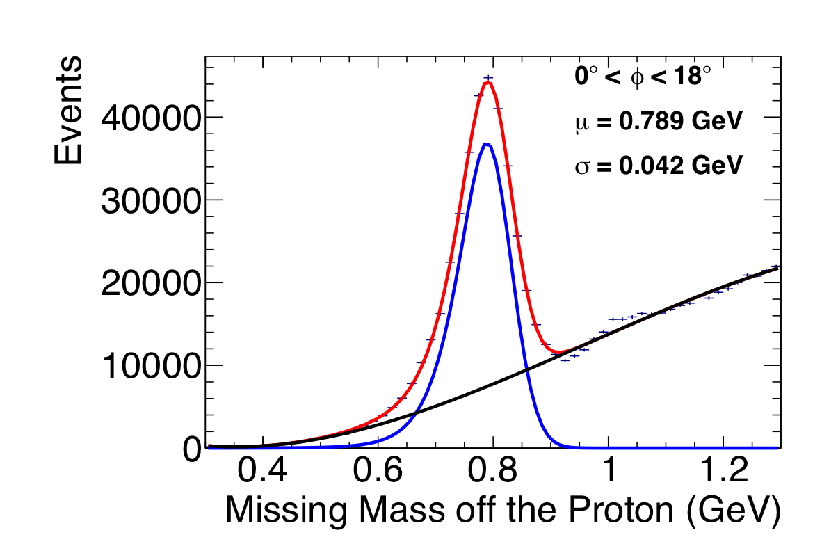
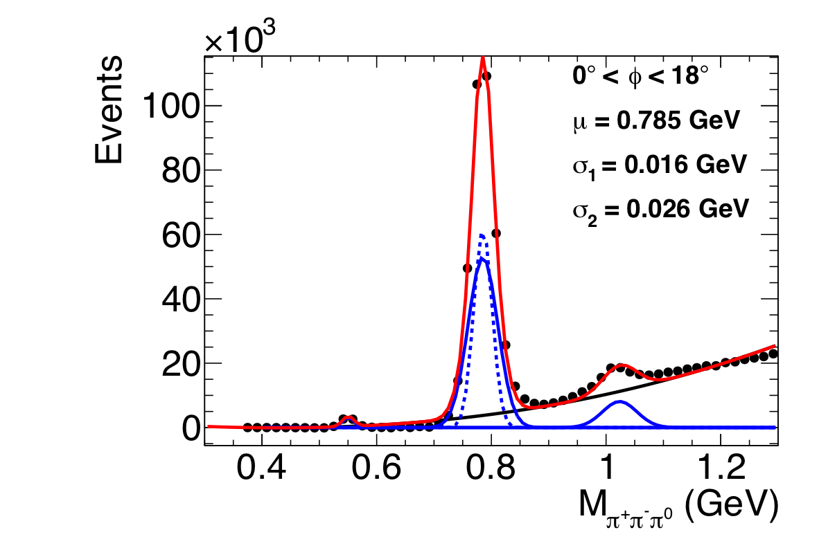
Figure 41a:
Reconstructed mass distributions for the reaction $\gamma p \to p\pi^0\pi^{\pm}(\pi^\mp)$ for a bin in $\phi$. (Left) Distribution of the missing mass off the proton. (Right) Invariant mass distribution for the $\pi^+\pi^-\pi^0$ system. The blue curves show the resonant contributions, the black curve show the polynomial backgrounds, and the red curve shows the sum. |
NIM A 987 (2021) 164807: downloads png pdf |
Figure 41b:
Reconstructed mass distributions for the reaction $\gamma p \to p\pi^0\pi^{\pm}(\pi^\mp)$ for a bin in $\phi$. (Left) Distribution of the missing mass off the proton. (Right) Invariant mass distribution for the $\pi^+\pi^-\pi^0$ system. The blue curves show the resonant contributions, the black curve show the polynomial backgrounds, and the red curve shows the sum. |
NIM A 987 (2021) 164807: downloads png pdf |
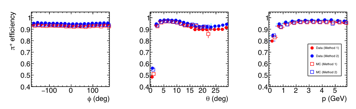
Figure 42:
Tracking efficiency for $\pi^+$ tracks, determined by data and simulation using two methods. |
NIM A 987 (2021) 164807: downloads png pdf |
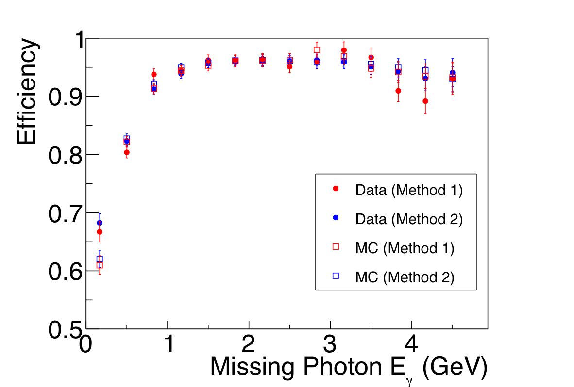
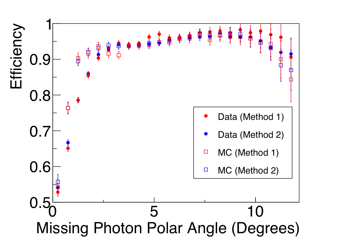
Figure 43a:
Photon reconstruction efficiency in FCAL determined from $\gamma p \to \omega p$, $\omega \to \pi^+\pi^-\pi^0$, $\pi^0 \to \gamma (\gamma)$ as a function of (left) photon energy and (right) photon polar angle. Good agreement between data and simulation is observed in the fiducial region $\theta = 2^\circ - 10.6^\circ$. |
NIM A 987 (2021) 164807: downloads png pdf |
Figure 43b:
Photon reconstruction efficiency in FCAL determined from $\gamma p \to \omega p$, $\omega \to \pi^+\pi^-\pi^0$, $\pi^0 \to \gamma (\gamma)$ as a function of (left) photon energy and (right) photon polar angle. Good agreement between data and simulation is observed in the fiducial region $\theta = 2^\circ - 10.6^\circ$. |

NIM A 987 (2021) 164807: downloads png pdf |
Figure 44:
Ratios of relative photon reconstruction efficiency between data and simulation determined from $\pi^0\to\gamma \gamma$ decays in $\gamma p \to \pi^+\pi^-\pi^0 p$ events. The efficiency ratios are shown for the cases where (left) both photons were measured in the BCAL, (middle) both photons were measured in the FCAL, and (right) one photon was measured in the BCAL and the other in the FCAL. |
NIM A 987 (2021) 164807: downloads png pdf |
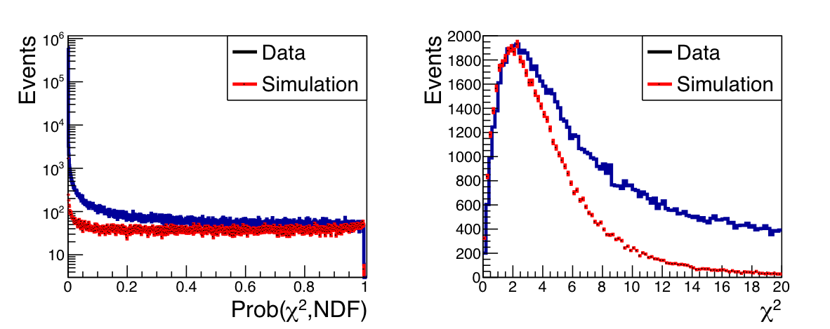
Figure 45:
Distribution of kinematic fit (left) probability and (right) $\chi^2$ for reconstructed $\gamma p \to \eta p$, $\eta \to \pi^+\pi^-\pi^0$ events in data and simulation. Both distributions agree reasonably for well-measured events, and diverge due to additional background in data and differences in modeling poorly-measured events. |
NIM A 987 (2021) 164807: downloads png pdf |
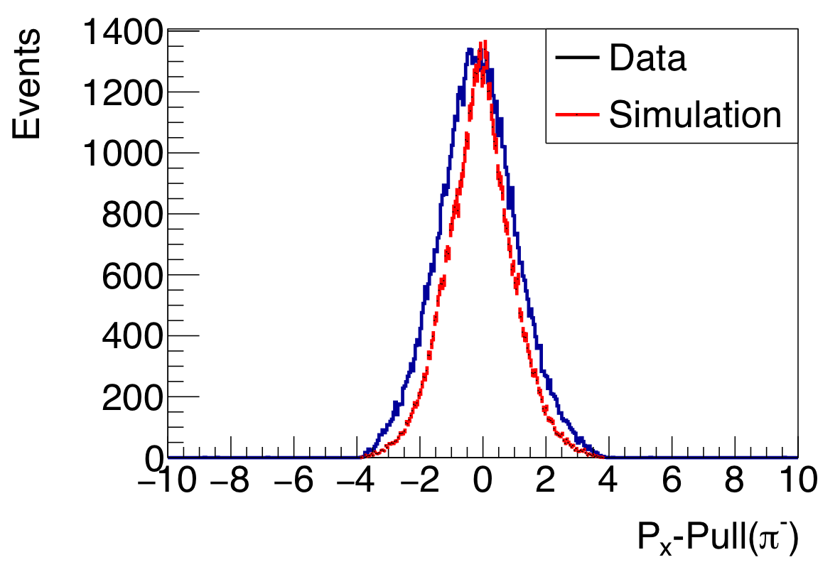
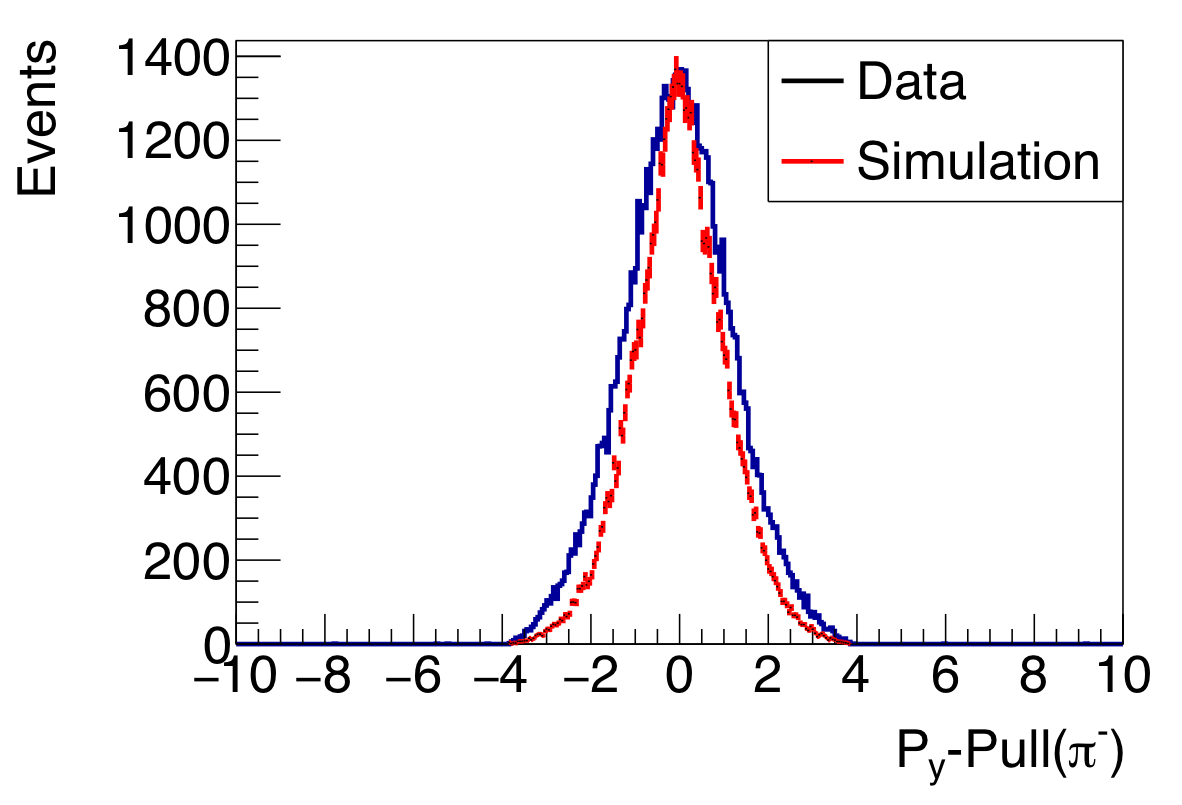
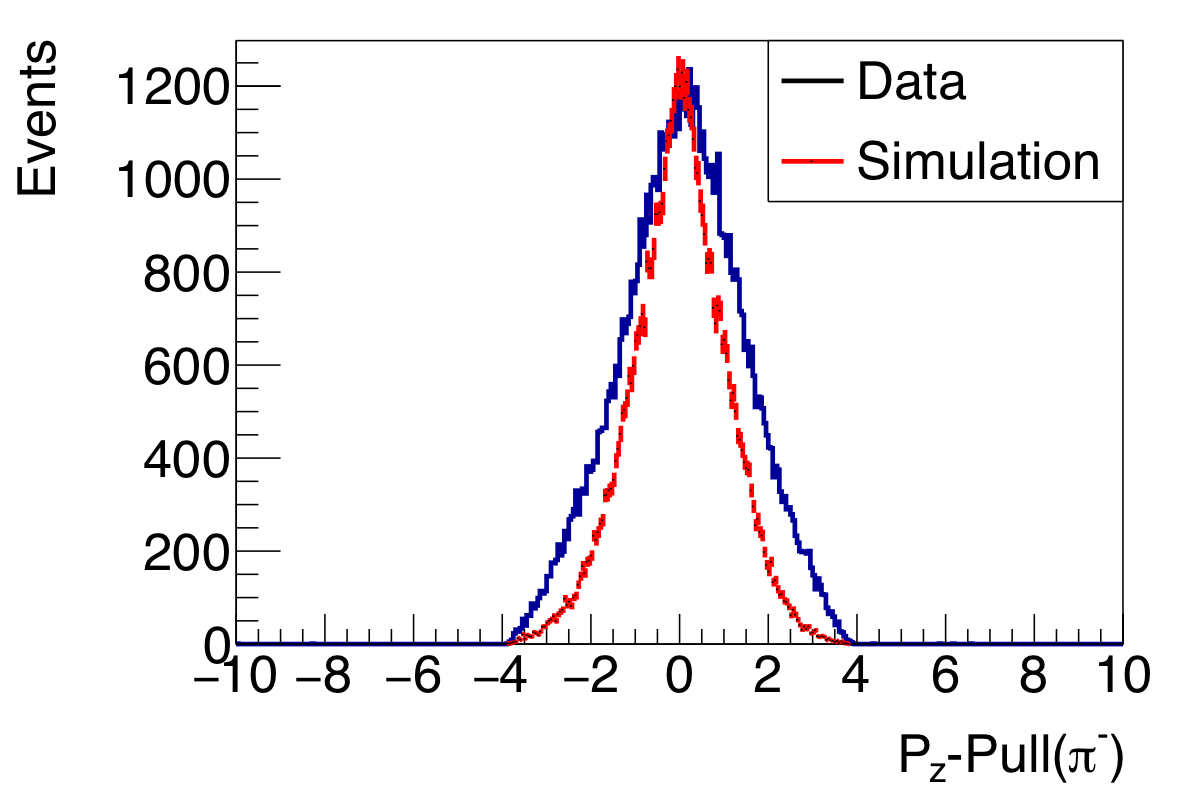
Figure 46a:
Pull distributions for momentum components of the $\pi^-$ from reconstructed $\gamma p \to \eta p$, $\eta \to \pi^+\pi^-\pi^0$ events in data and simulation for events with fit probability $>0.01$, (left) $p_x$, (center) $p_y$, (right) $p_z$. |
NIM A 987 (2021) 164807: downloads png pdf |
Figure 46b:
Pull distributions for momentum components of the $\pi^-$ from reconstructed $\gamma p \to \eta p$, $\eta \to \pi^+\pi^-\pi^0$ events in data and simulation for events with fit probability $>0.01$, (left) $p_x$, (center) $p_y$, (right) $p_z$. |
NIM A 987 (2021) 164807: downloads png pdf |
Figure 46c:
Pull distributions for momentum components of the $\pi^-$ from reconstructed $\gamma p \to \eta p$, $\eta \to \pi^+\pi^-\pi^0$ events in data and simulation for events with fit probability $>0.01$, (left) $p_x$, (center) $p_y$, (right) $p_z$. |

NIM A 987 (2021) 164807: downloads png pdf |
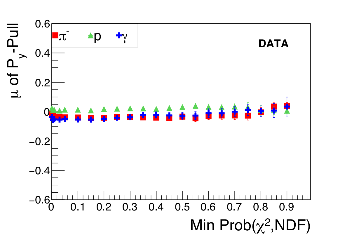
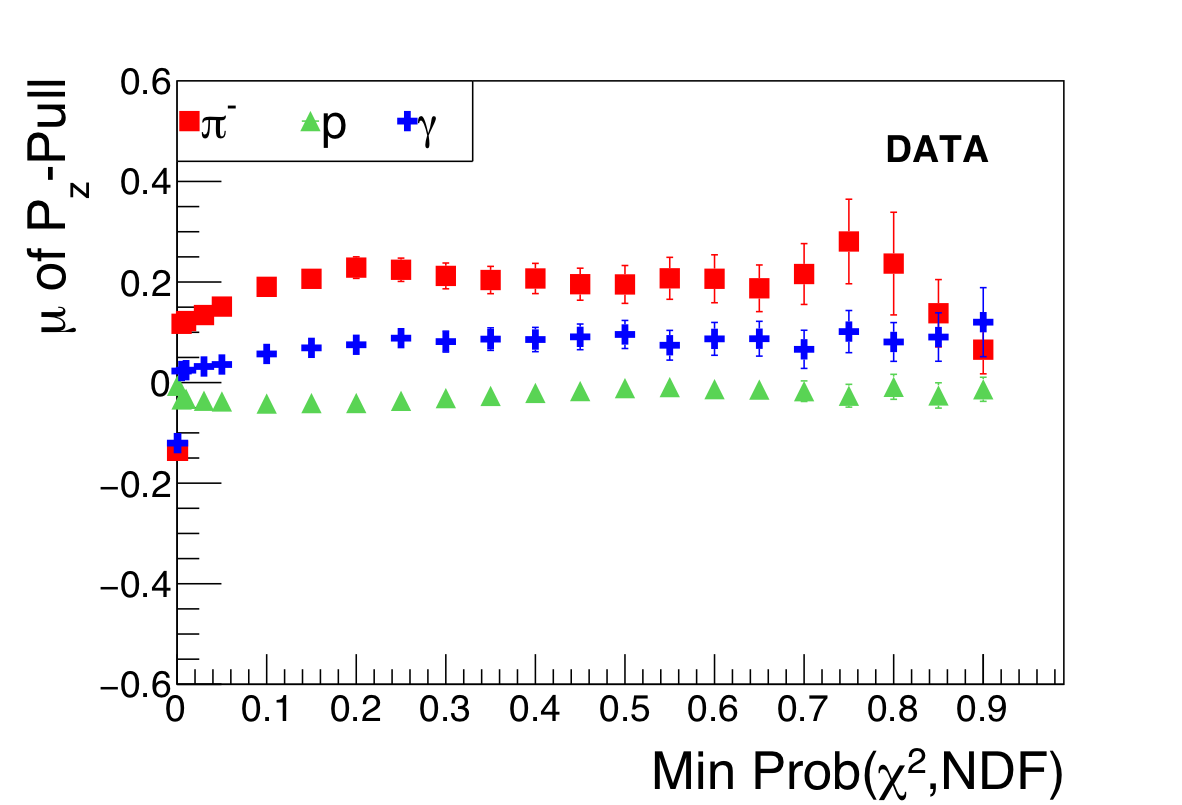
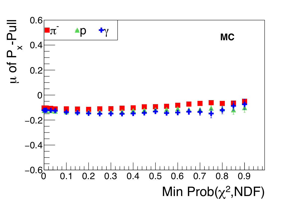
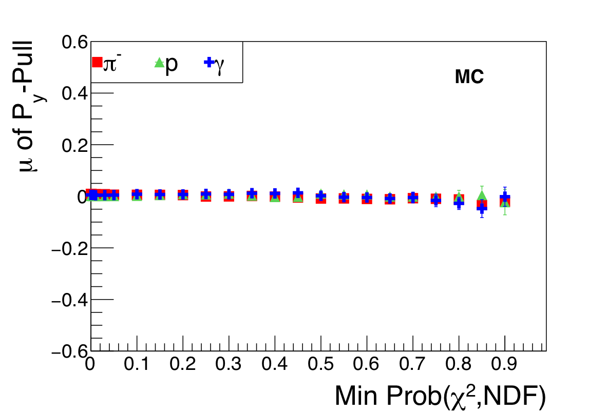
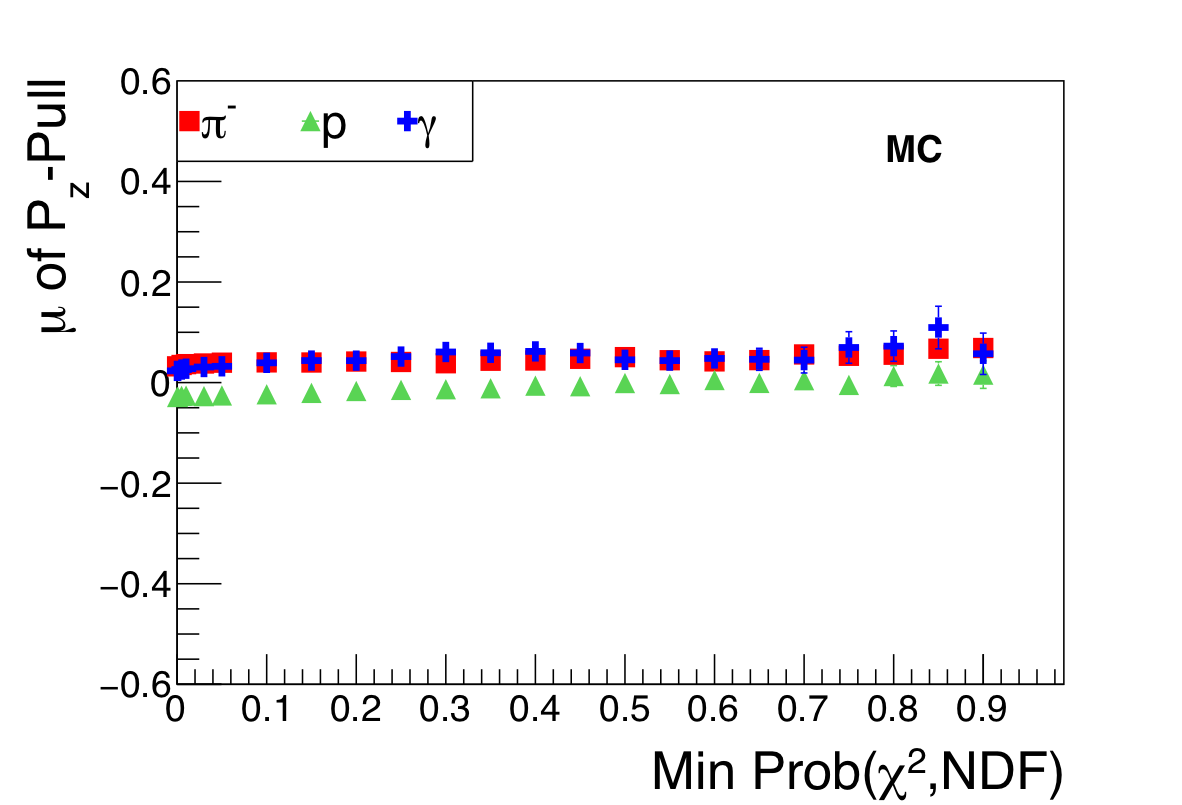
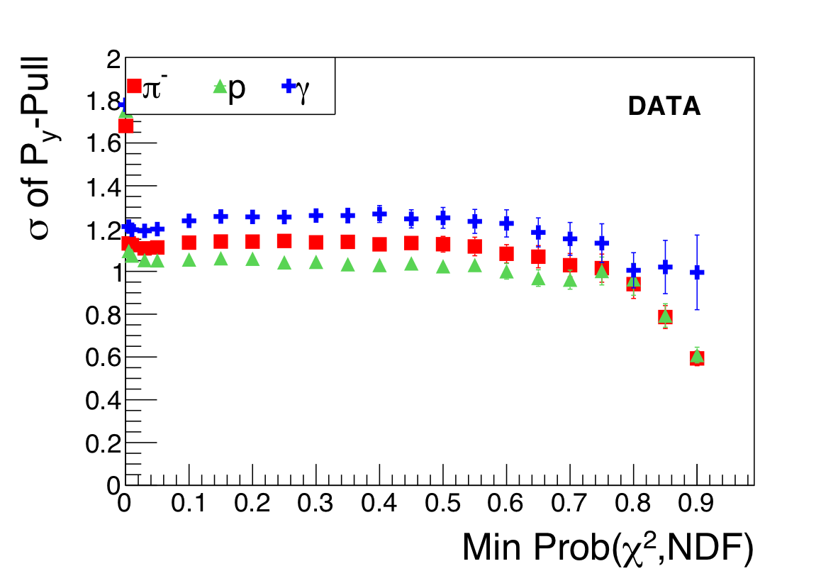
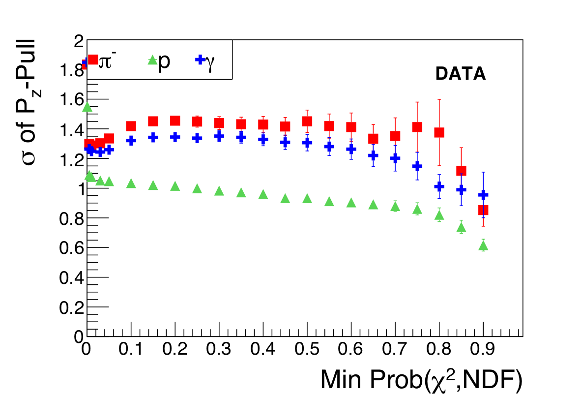
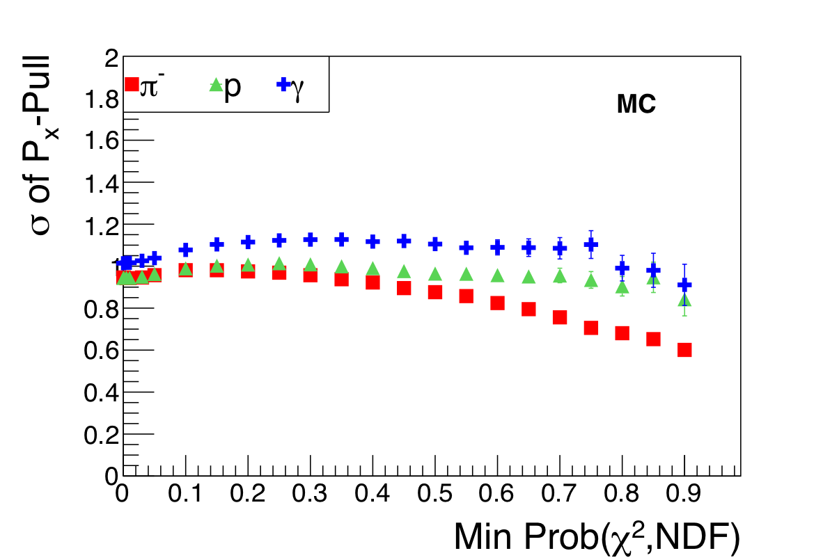
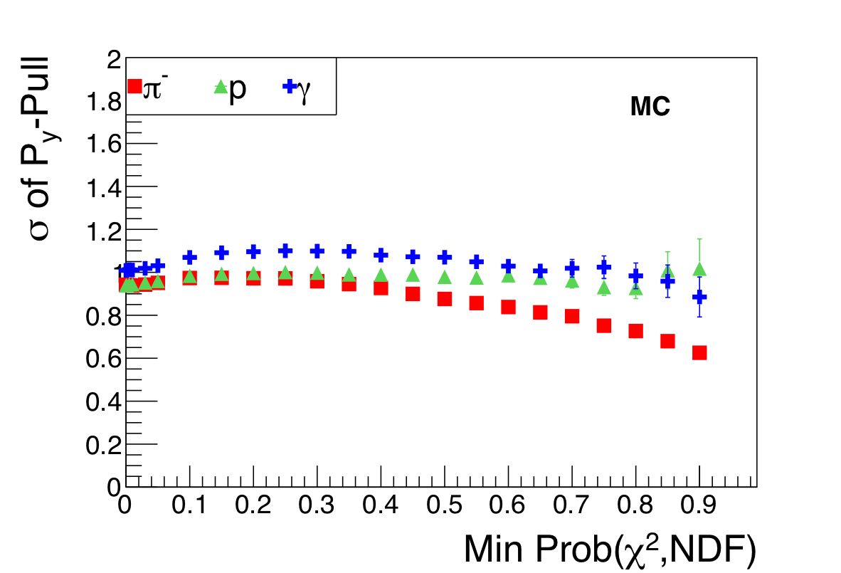
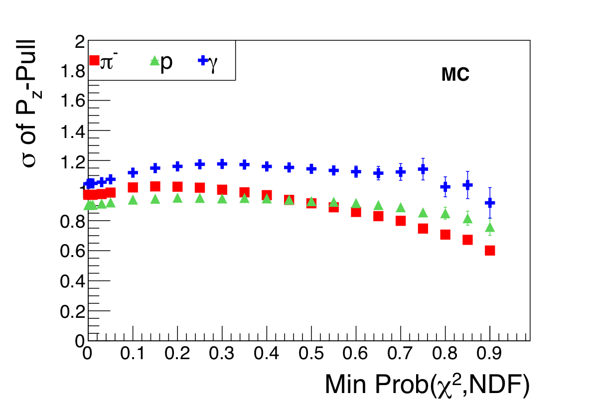
Figure 47a:
Pull means (top) and sigmas (bottom) for the momentum components of each particle as a function of the minimum probability required of the fit from reconstructed $\gamma p \to \eta p$, $\eta \to \pi^+\pi^-\pi^0$ events. |
NIM A 987 (2021) 164807: downloads png pdf |
Figure 47b:
Pull means (top) and sigmas (bottom) for the momentum components of each particle as a function of the minimum probability required of the fit from reconstructed $\gamma p \to \eta p$, $\eta \to \pi^+\pi^-\pi^0$ events. |
NIM A 987 (2021) 164807: downloads png pdf |
Figure 47c:
Pull means (top) and sigmas (bottom) for the momentum components of each particle as a function of the minimum probability required of the fit from reconstructed $\gamma p \to \eta p$, $\eta \to \pi^+\pi^-\pi^0$ events. |
NIM A 987 (2021) 164807: downloads png pdf |
Figure 47d:
Pull means (top) and sigmas (bottom) for the momentum components of each particle as a function of the minimum probability required of the fit from reconstructed $\gamma p \to \eta p$, $\eta \to \pi^+\pi^-\pi^0$ events. |
NIM A 987 (2021) 164807: downloads png pdf |
Figure 47e:
Pull means (top) and sigmas (bottom) for the momentum components of each particle as a function of the minimum probability required of the fit from reconstructed $\gamma p \to \eta p$, $\eta \to \pi^+\pi^-\pi^0$ events. |
NIM A 987 (2021) 164807: downloads png pdf |
Figure 47f:
Pull means (top) and sigmas (bottom) for the momentum components of each particle as a function of the minimum probability required of the fit from reconstructed $\gamma p \to \eta p$, $\eta \to \pi^+\pi^-\pi^0$ events. |

NIM A 987 (2021) 164807: downloads png pdf |
Figure 47g:
Pull means (top) and sigmas (bottom) for the momentum components of each particle as a function of the minimum probability required of the fit from reconstructed $\gamma p \to \eta p$, $\eta \to \pi^+\pi^-\pi^0$ events. |
NIM A 987 (2021) 164807: downloads png pdf |
Figure 47h:
Pull means (top) and sigmas (bottom) for the momentum components of each particle as a function of the minimum probability required of the fit from reconstructed $\gamma p \to \eta p$, $\eta \to \pi^+\pi^-\pi^0$ events. |
NIM A 987 (2021) 164807: downloads png pdf |
Figure 47i:
Pull means (top) and sigmas (bottom) for the momentum components of each particle as a function of the minimum probability required of the fit from reconstructed $\gamma p \to \eta p$, $\eta \to \pi^+\pi^-\pi^0$ events. |
NIM A 987 (2021) 164807: downloads png pdf |
Figure 47j:
Pull means (top) and sigmas (bottom) for the momentum components of each particle as a function of the minimum probability required of the fit from reconstructed $\gamma p \to \eta p$, $\eta \to \pi^+\pi^-\pi^0$ events. |
NIM A 987 (2021) 164807: downloads png pdf |
Figure 47k:
Pull means (top) and sigmas (bottom) for the momentum components of each particle as a function of the minimum probability required of the fit from reconstructed $\gamma p \to \eta p$, $\eta \to \pi^+\pi^-\pi^0$ events. |
NIM A 987 (2021) 164807: downloads png pdf |
Figure 47l:
Pull means (top) and sigmas (bottom) for the momentum components of each particle as a function of the minimum probability required of the fit from reconstructed $\gamma p \to \eta p$, $\eta \to \pi^+\pi^-\pi^0$ events. |
NIM A 987 (2021) 164807: downloads png pdf |
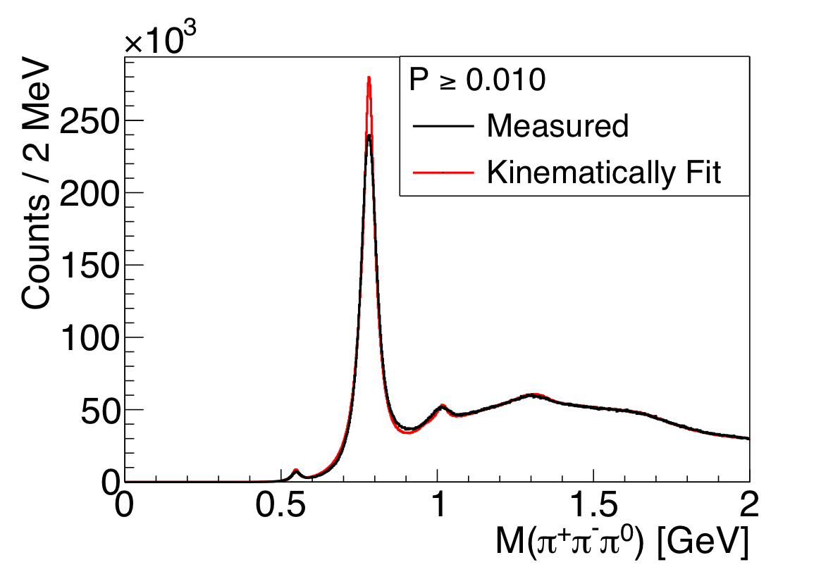
Figure 48a:
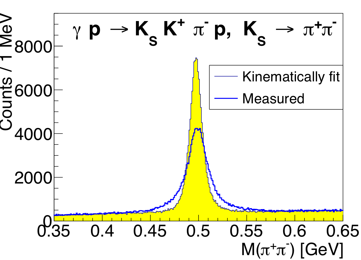
(Left) $\pi^+\pi^-\pi^0$ invariant-mass distribution from $\gamma p \to \pi^+\pi^-\pi^0 p$ (Right) $\pi^+\pi^-$ invariant mass distribution from $\gamma p \to K_S K^+ \pi^- p$, $K_S\to\pi^+\pi^-$. |
NIM A 987 (2021) 164807: downloads png pdf |
Figure 48b:
(Left) $\pi^+\pi^-\pi^0$ invariant-mass distribution from $\gamma p \to \pi^+\pi^-\pi^0 p$ (Right) $\pi^+\pi^-$ invariant mass distribution from $\gamma p \to K_S K^+ \pi^- p$, $K_S\to\pi^+\pi^-$. |
NIM A 987 (2021) 164807: downloads png pdf |
Figure 49:
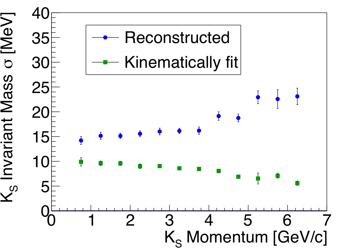
$K_S\to\pi^+\pi^-$ invariant mass resolution for the events shown in Fig. 48, as a function of $K_S$ momentum, both before and after a kinetic fit, which constrains energy and momentum conservation. |
NIM A 987 (2021) 164807: downloads png pdf |
Figure 50a:
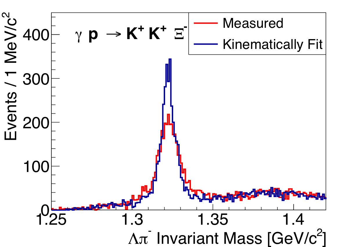
(Left) $\Lambda^0\pi^-$ invariant mass distribution from $\gamma p \to K^+ K^+ \pi^- \pi^- p$. (Right) $e^+e^-$ invariant mass distribution from kinematically fit $\gamma p \to e^+e^- p$ events. |

NIM A 987 (2021) 164807: downloads png pdf |
Figure 50b:
(Left) $\Lambda^0\pi^-$ invariant mass distribution from $\gamma p \to K^+ K^+ \pi^- \pi^- p$. (Right) $e^+e^-$ invariant mass distribution from kinematically fit $\gamma p \to e^+e^- p$ events. |

NIM A 987 (2021) 164807: downloads png pdf |
Figure 51:
CDC energy loss ($dE/dx$) for positively charged particles that have at least 20 hits in the detector, as a function of measured particle momentum. The band corresponding to protons curves upwards, showing a larger energy loss than pions and other lighter particles at low momentum. The two bands show a clear separation for momenta $\lesssim 1$ GeV. A faint kaon band can be seen between them. |
NIM A 987 (2021) 164807: downloads png pdf |
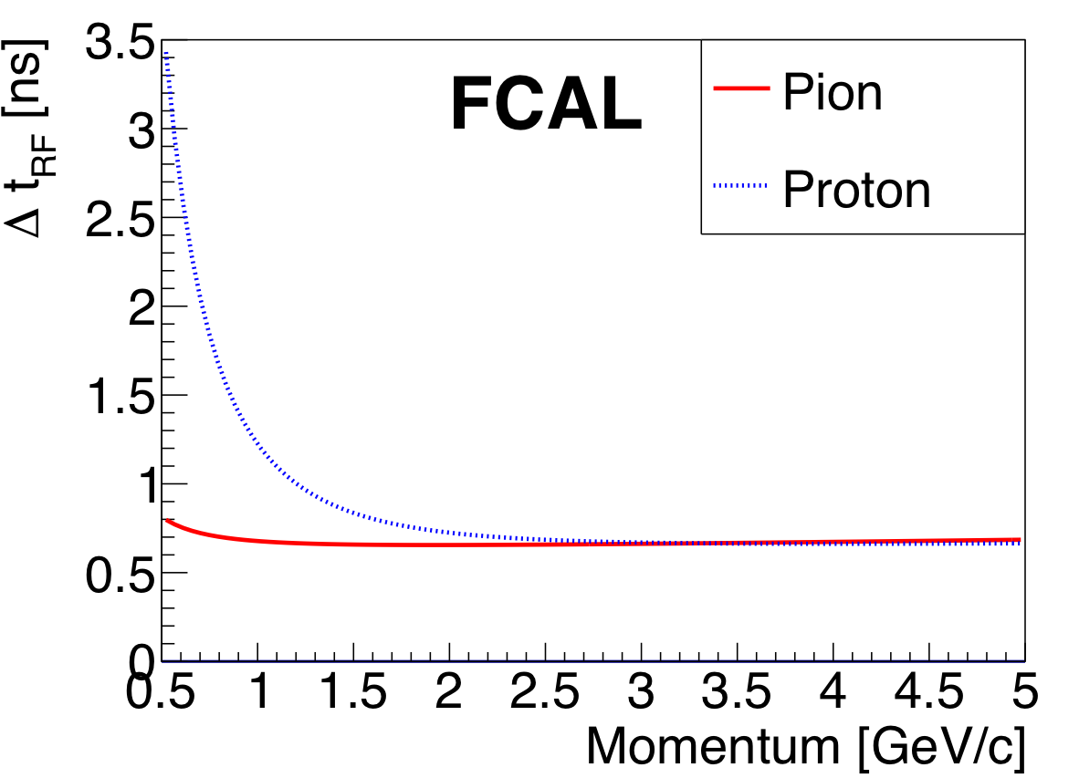
Figure 52a:
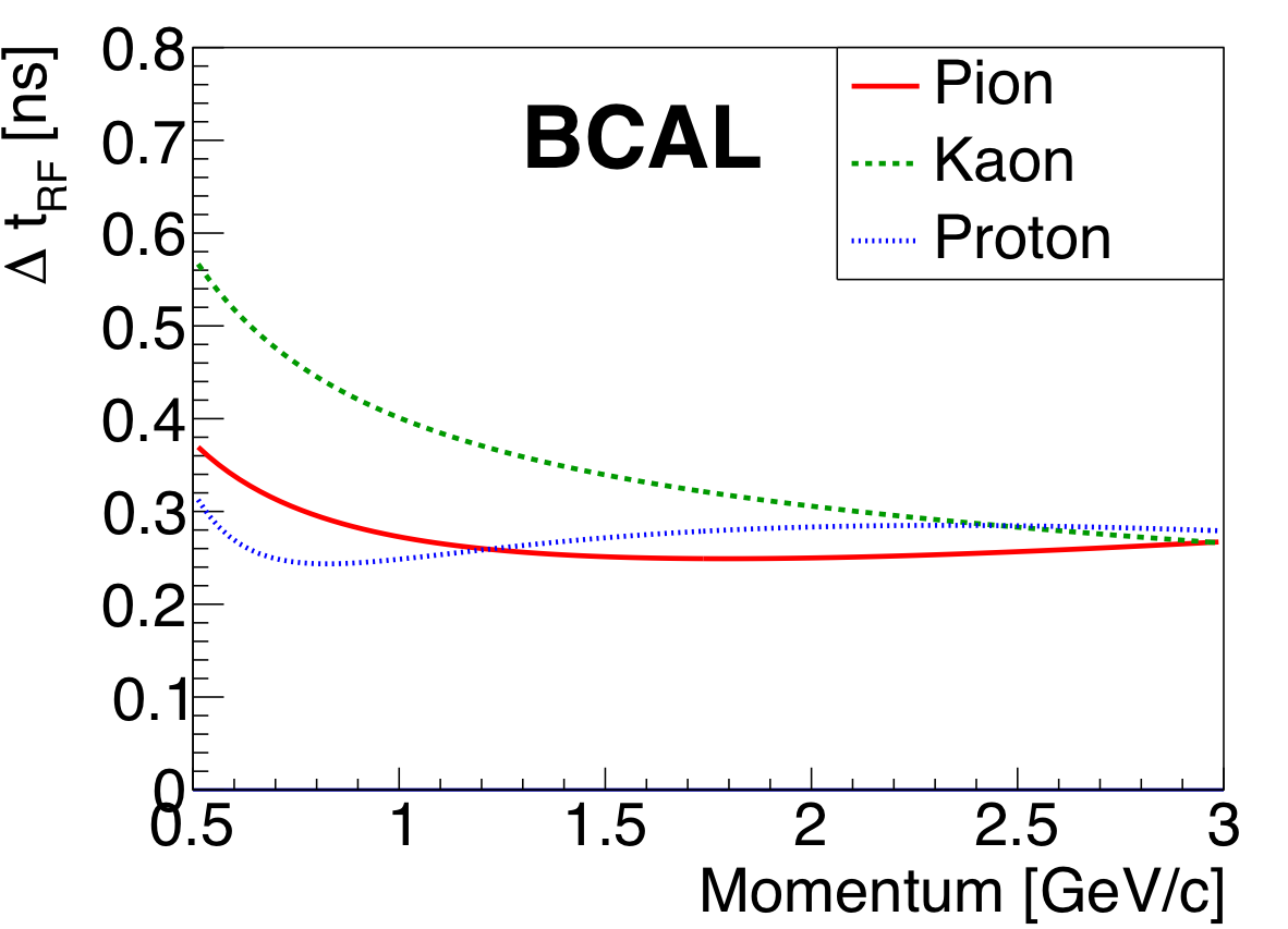
Resolution as a function of particle momentum for $\Delta t_\mathrm{RF}$ in various subdetectors, (left) BCAL, (center) FCAL, (right) TOF |
NIM A 987 (2021) 164807: downloads png pdf |
Figure 52b:
Resolution as a function of particle momentum for $\Delta t_\mathrm{RF}$ in various subdetectors, (left) BCAL, (center) FCAL, (right) TOF |

NIM A 987 (2021) 164807: downloads png pdf |
Figure 52c:
Resolution as a function of particle momentum for $\Delta t_\mathrm{RF}$ in various subdetectors, (left) BCAL, (center) FCAL, (right) TOF |
NIM A 987 (2021) 164807: downloads png pdf |
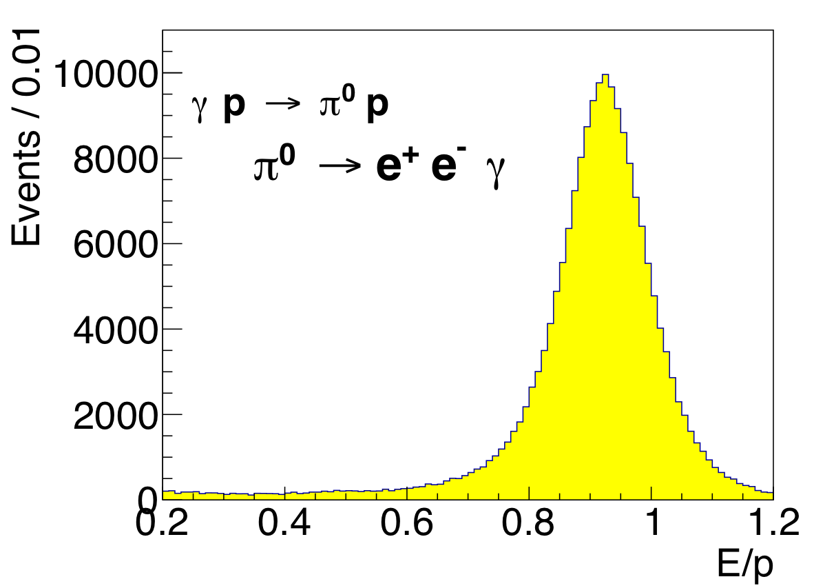
Figure 53a:
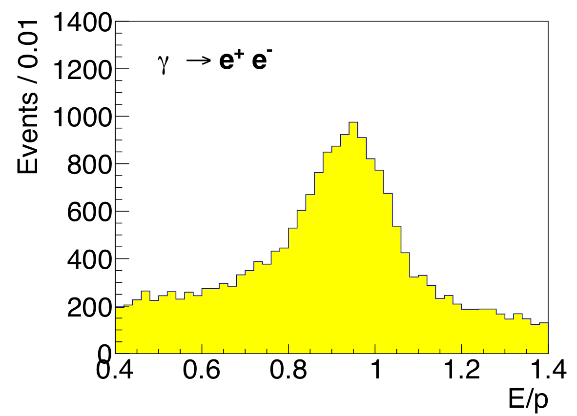
Electron identification in the calorimeters is performed using the $E/p$ variable, the ratio of the energy loss in the electromagnetic calorimeters ($E$) to the momentum reconstructed in the drift chambers ($p$). Left) This distribution was obtained using $e^{\pm}$ showers reconstructed in the FCAL from the reaction $\gamma p \to \pi^0 p$, $\pi^0\to e^+e^-\gamma$. Right) $e^{\pm}$ showers reconstructed in the BCAL from photon conversions. |
NIM A 987 (2021) 164807: downloads png pdf |
Figure 53b:
Electron identification in the calorimeters is performed using the $E/p$ variable, the ratio of the energy loss in the electromagnetic calorimeters ($E$) to the momentum reconstructed in the drift chambers ($p$). Left) This distribution was obtained using $e^{\pm}$ showers reconstructed in the FCAL from the reaction $\gamma p \to \pi^0 p$, $\pi^0\to e^+e^-\gamma$. Right) $e^{\pm}$ showers reconstructed in the BCAL from photon conversions. |
NIM A 987 (2021) 164807: downloads png pdf |
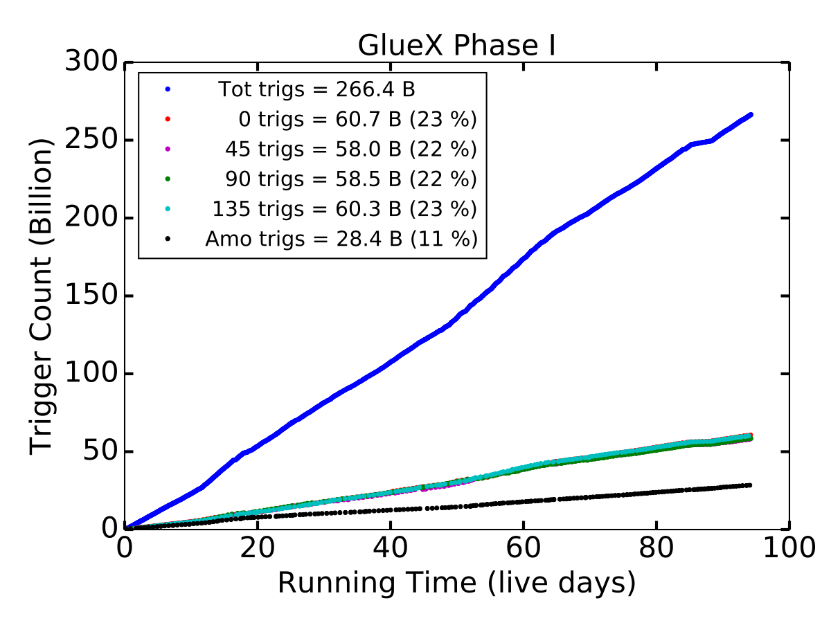
Figure 54:
Plot of integrated number of triggers versus the number of live days in 2017 and 2018. The legend provides the number of triggers for the four diamond orientations relative to the horizontal (0, 45, 90, 135$^\circ$) and the amorphous radiator. The trigger curves of the four diamond configurations fall on top of one another, as we attempted to match the amount of data taken for each configuration. |